Lab 3

Lossy compression

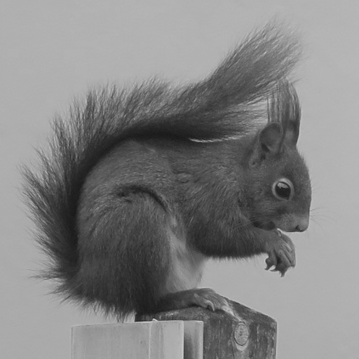
The heart of JPEG compression is to save the low-frequency coefficients of the discrete cosine transform (DCT) of the image with low precision. In this exercise, a simplified version of JPEG compression is implemented by cancelling the DCT pixels located outside a certain frequency.

• Compute and display the DCT (scipy.fftpack.dctn with argument norm='ortho') of the image squirrel.png.

• Apply a binary mask to the DCT coefficients to cancel the high frequencies.The Recall that for DCT, the low frequencies are located at the top left corner of the image.

• Display the compressed image using reverse DCT (scipy.fftpack.idctn, always with the argument norm='ortho'). What is your opinion about the quality of the compression?

• Calculate the mean square error (MSE) defined as:

  \[ MSE = \frac{1}{MN} \sum_ {m,n} (f(m,n) - g(m,n))^2 \]

  where \(f\) and \(g\) are respectively the images before and after compression, \(M\) and \(N\) being the dimensions of these images. You can use the function numpy.linalg.norm.

• Analyze the evolution of the MSE according to the mask size.

Interpolation

The difference between different interpolation methods will be observed by applying successive rotations on the image chess.png. The rotations will be made by using skimage.transform.rotate, which permits to choose different interpolation approaches.

• Perform four successive rotations of 90° of the image, and observe the effect of the rotation at each step. Use the default value for each parameter.

• Compare the resulting image with the original one, both visually and using the MSE.

• Now perform nine rotations of 40° and compare with the original image. What do you observe?

• Compare the previous result with other interpolation methods.