Filtering aliasing

Objectives

• Define and apply a filter for a real application

• Discover aliasing in images

Warning: because Jupyter Lab and Matplotlib show images with a rescaling, the function imshow can introduce aliasing, even if there is no aliasing in the actual image. Therefore, do not use imshow in this exercice, but save the image (with skimage.io.imsave) and display it by using an external viewer.

Downsampling and filtering

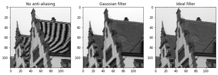
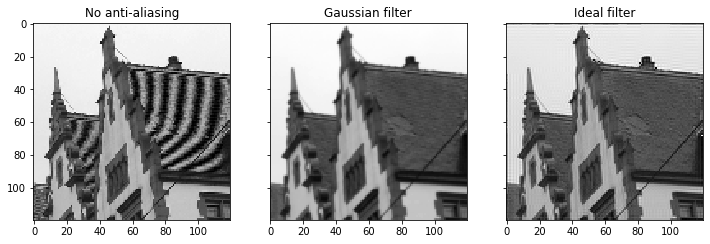
Three images are generated:

• the original one, rescaled by a factor \(S\),

• the original one, filtered by a Gaussian filter, then rescaled by a factor \(S\),

• the original one, filtered by an ideal low-pass filter (defined in the Fourier domain), then rescaled by a factor \(S\).

Note that when using the inverse Fourier transform, you may have to get the real part of the result, if it is complex.

The mask is of the same size that the Fourier transform X of the original image. The low frequencies must be 1 and the high frequency 0, as in the image below (the pixels 1 are in the center to manage the use of fftshift):

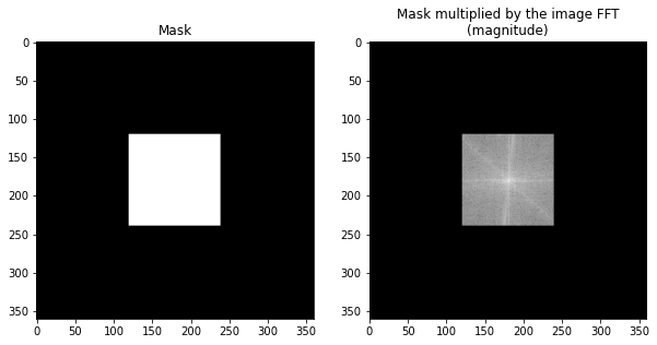
Note that the cutoff frequency equals \(1/S\) to avod aliasing.

You should obtain the following results. The aliasing is clearly visible on the first image, where no filter has been applied: a weird effect is visible on the tiles. The Gaussian filter strongly attenuates the effect, and the ideal filter is better.