Mathematical morphology#
Objectives#
apply and compare basic operations (erosion, dilation, opening, closing)
evaluate of the parameters of these operations
use connected components to extract useful information
First processings#
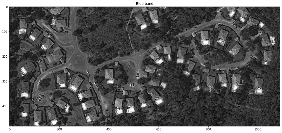
The image is a satellite view of a small town in the Landes, France. It is an RGB image of resolution 50 cm.
Since the objects of interest are blue and no other object in the scene is of this color, it may be interesting to deal with the blue band of the image. Therefore, the pools are bright on the blue band, giving first discrimination between the pools and the rest.
blue = img[:,:,2]
The mathematical morphology operators described in the course work on binary images. The blue band can be binarized by applying a threshold to separate the bright pixels from the others. By looking at the histogram of the blue band and proceeding by trial and error, we choose a threshold equals to 240.
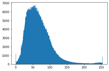
cropbinarized = (blue > 240)
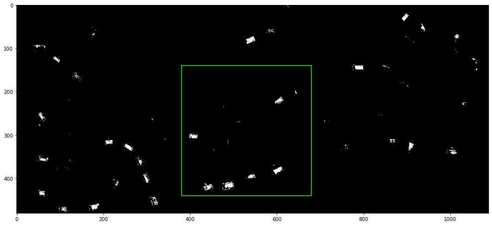
Study of the different operators#
In this part, the mathematical morphology operators are applied to the sub-image marked out by the green square on the image above.
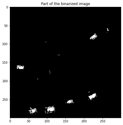
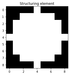
First of all, we choose as a structuring element a disk with a radius of 4 pixels.
The four basic operators applied to the image produce the results below.
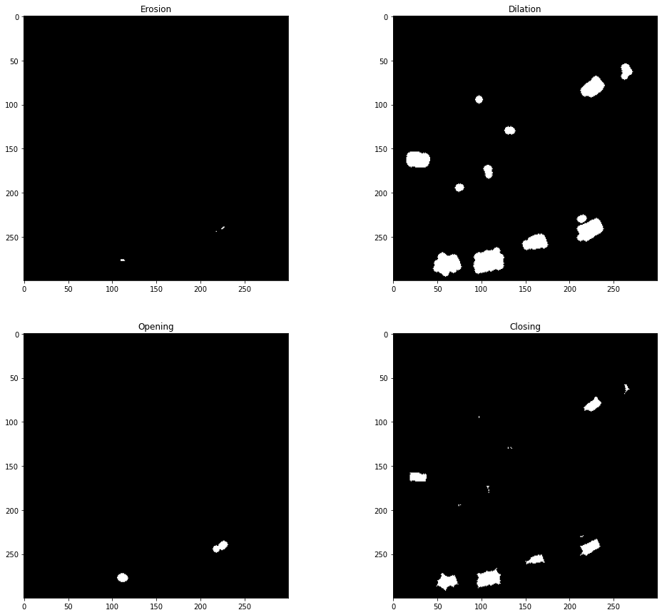
Which operator(s) tend(s) to plug the holes?
On the contrary, which operator(s) tend(s) to remove small objects?
Which operator(s) preserve(s) (roughly) the shape of objects?
The same with a 10-pixel radius disk:
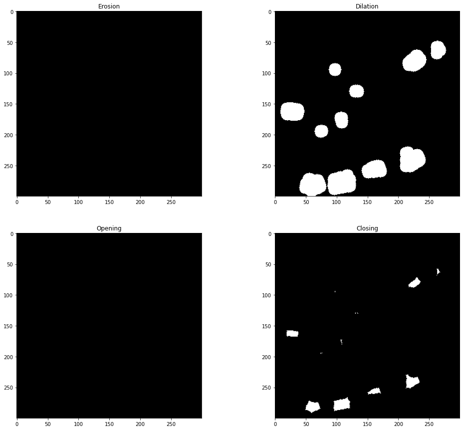
Try other structuring elements to observe their influence!
Pool detection#
In the following, we consider the result of a closing with a 10-pixel radius disk for structuring element.
The function skimage.morphology.label returns a labeling of the different connected components,
and the function skimage.measure.regionprops measure some geometric properties of the connected components,
such as their surface or their position.
Number of connected component (that is, detected pools): 69
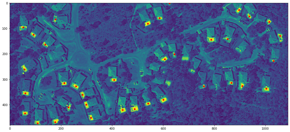
The centroids of the connected components are represented in the image below by the red dots.
Of course, there are fewer pools than red dots, but a lot of connected components are actually small groups of pixels that do not correspond to pools.
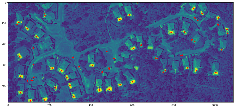
The result can be improved by considering only the connected components whose number of pixels is greater than a certain value. So, we have chosen to consider as pools the connected components whose area is greater than 20 pixels.
Moreover, we know that a pixel represents an area of 0.5\(\times\)0.5 m2, so it is easy to calculate the average area of the detected pools.
Number of detected pools: 36
Average area of the detected pools: 40.89 m²
Discussion#
The method proposed in this notebook is simple but not robust: swimming pools shaded or partially hidden by a tree are not always detected. Conversely, some objects can be considered as swimming pools because they are very bright in the blue band and large. Therefore, some improvements to improve the result are listed below:
The geometry of the connected components can be considered because the swimming pools are not only blue objects with a sufficiently large area, but they also have a rectangular shape;
we choose the threshold for binarization to work well on this image. But nothing guarantees that this value can be applied to another image: it may depend on the sensor resolution, the image brightness, the type of swimming pool, etc. In other words, the robustness of the threshold value has to be studied.
the binarization of the image could take into account the binarization of the neighbouring pixels. This principle can be modelled using Markov fields.
etc.