Lossy compression

Objectives

• know how to implement the basic principle of JPEG compression

• use the discrete cosine transform

• analyze the effect of compression on visual quality and PSNR

Images of the DCT basis

First of all, it is interesting to view the elements of the DCT basis.

Since the images of the base correspond to a single non-zero coefficient in the domain of the transform, a solution to display these images is to create images that are zero in the domain of the transform, except in a single pixel. By using the function scipy.fftpack.idctn, we can get the corresponding 2D cosine. The low frequencies are at the top left.

Here are some examples of images of the base (on the first line) and their DCT (on the second line) for a size of 8 × 8 pixels.

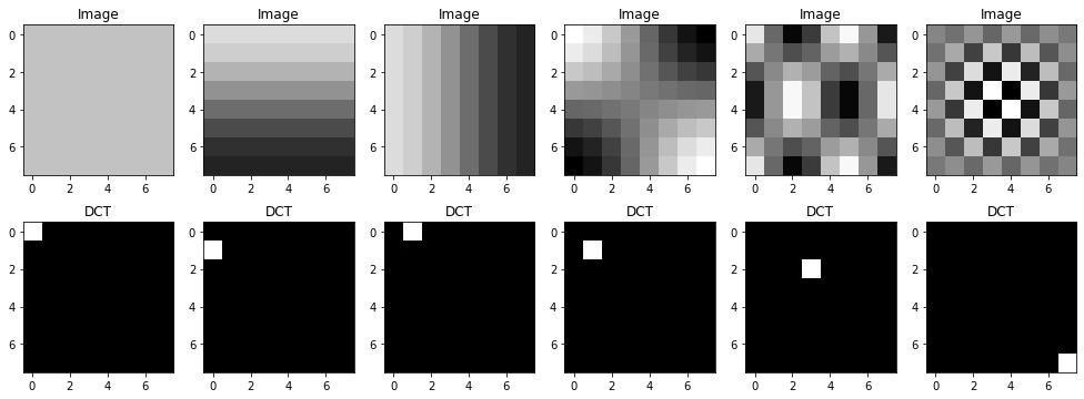
It can be seen that the pixels at the top left of the DCT (therefore close to the origin) correspond to a low-frequency since the corresponding image is a 2D cosine of low frequency in the spatial domain. Conversely, the pixel at the bottom right is the very high frequency component: the intensity of the pixels changes very quickly in the image.

Application of the JPEG principle

Unlike the Fourier transform which decomposes an image as complex exponentials, the DCT decomposes an image as real cosines. Therefore the result is not complex; there is no need to display modulus and phase. Yet, the zero frequency coefficient being much greater than the others, the contrast of the DCT must be modified (how?) to visualize it.

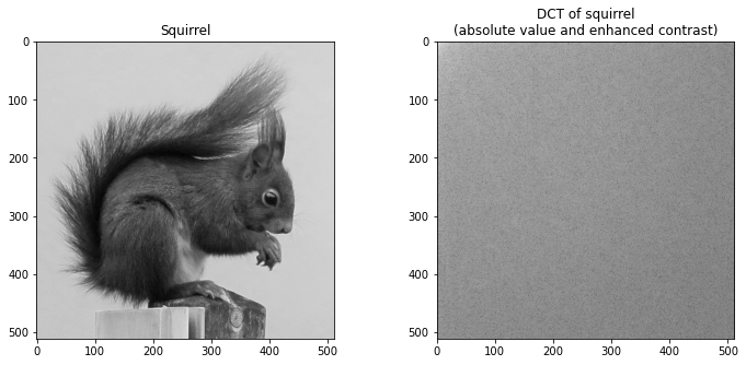
We can notice (even if it is not obvious) that the low-frequency coefficients are more energetic than the others. This means that the image is mostly made up of low frequencies.

To perform the compression, we choose to cancel the high-frequency pixels using a square mask of side \(C\). The size of the square divided by the image size corresponds to the compression ratio.

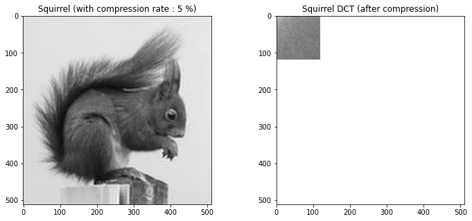
Note that even with a low compression ratio, the visual result is very good: it is very difficult to observe the differences between the two images. This observation is also confirmed by the low value of the MSE:

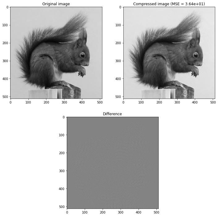
The difference image is interesting because we can see that the errors are mainly located in the areas of high frequencies (contours, tail…). This makes sense since it is precisely these high frequencies that have been cancelled.

JPEG compression plays on the fact that the human eye is not sensitive to these high-frequency changes.

MSE evolution

The previous procedure is now used with different size of the mask, in order to calculate the MSE between the compressed image and the original image. The PSNR is also indicated, it is a measure that we will see in a future course.

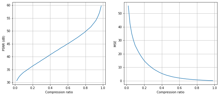
The analysis of the curves leads to the following conclusions.

• The larger the PSNR, the better the picture quality: so it makes sense that it increases as the compression ratio increases.

• Conversely, MSE measures the difference between the compressed image and the original image: as the compression ratio increases, the difference becomes smaller and smaller, so the MSE decreases.

In classic JPEG compression, the DCT is not directly calculated on the whole image, but on 8 × 8 size thumbnails, as is done below.

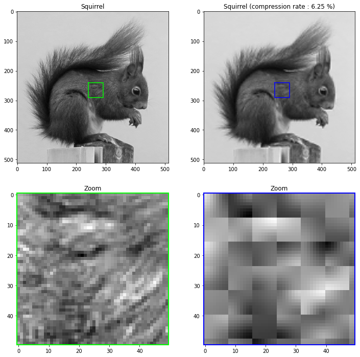
Compression on 8×8 sub-images

The image is divided into blocks of 8×8 pixels, then the DCT is computed on each block, and finally, the high frequencies of each DCT are cancelled. The blocking effect is clearly visible when the compression is too strong.