Convolution

Objectives

• know how to use the function scipy.ndimage.convolve to apply the convolution product

• be able to identify the kernel applied on a convolved image

The point spread functions

Before convolving the image by the different filters, it is interesting to display the filters themselves. In case there is no explicit matrix to represent a filter, as with the Gaussian filter skimage.filters.gaussian, we can simply convolve the filter by an image containing only one non-zero pixel. Indeed, this image is equivalent to a Dirac pulse \(\delta\) which is the neutral element of the convolution product.

The two last kernels are defined with (note the double brackets, so as to get a 2D array):

h = np.array([[1, -1]])

and

N = 30
h = np.ones((1,N)) / N

The convolutions

The results of the convolutions are shown below, for both the “Dirac pulse” and the smiley.

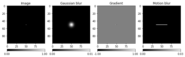
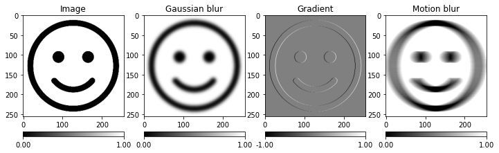
The function skimage.filters.gaussian defines a Gaussian kernel (this is the second image above). The result of the function is the convolution product of this Gaussian kernel with the image given as a parameter of the function.

The “gradient” image (third image) brings out the vertical contours of the image. We will reuse this filter in Edge detection.

import matplotlib.pyplot as plt
import numpy as np

img = np.arange(100).reshape((10, 10))/100

plt.figure()
im = plt.imshow(img, "gray")
plt.colorbar(im)
plt.show()