Denoising

The objectives of this exercise are:

• to apply a white Gaussian noise with a specific SNR on an image

• to implement a denoising method

• to understand the effects of the parameters and set it accordingly to the epexpected solution

Two denoising methods are considered in this correction: the mean filter and TV regularization.

Original image and noisy image

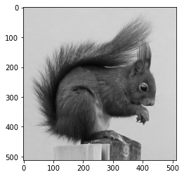
The original image:

<matplotlib.image.AxesImage at 0x7fd6a07a3c40>

The signal-to-noise ratio (SNR) is defined as the power of the image \(x\) divided by the power of the noise \(b\). Besides, it is generally given with a logarithmic scale.

\[ \mathrm{SNR} = 10 \log_{10} \left(\frac{P_x}{P_b}\right) \quad\Leftrightarrow\quad 10^\frac{\mathrm{SNR}}{10} = \frac{P_x}{P_b} \]

where:

\[ Px = \frac{1}{MN} \sum_{m,n} x(m,n)^2 \quad\text{et}\quad Pb = \frac{1}{MN} \sum_{m,n} b(m,n)^2 = \sigma^2 \]

Then:

\[\begin{split} &P_b = \frac{P_x}{10^\frac{\mathrm{SNR}}{10}} \\ \Leftrightarrow\quad &\sigma^2 = P_x \times 10^{-\frac{\mathrm{SNR}}{10}} \\ \Leftrightarrow\quad &\sigma^2 = \frac{1}{MN} \sum_{m,n} x(m,n)^2 10^{-\frac{\mathrm{SNR}}{10}} \\ \end{split}\]

Note that \(\sqrt{\sum_{m,n} x(m,n)^2} \) corresponds to the Frobenius norm of \(x\) and can be calculated with numpy.linalg.norm.

The figures below represent the image at different noise levels.

Warning: do not forget clip=False when using skimage.util.random_noise, in order to add a true Gaussian noise!

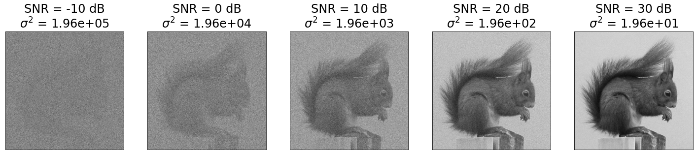
Note that the larger the SNR, the less visible the noise. This makes sense since, in the definition of SNR, the noise power is in the denominator. In addition, the noise becomes almost invisible beyond 30 dB, while it is very high and the image is hardly visible below 0 dB.

Mean filter

I choose the image whose SNR equals 10 dB, and I apply a mean filter.

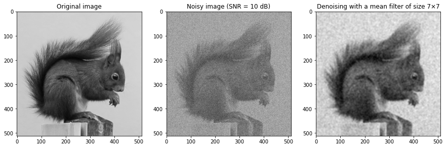
We observe that the mean filter reduces the noise, which is expected (have you tried a filter of size 1×1? What’s going on?). On the other hand, the image is more blurry: the contours are less sharp. This second observation is explained by the fact that the mean filter is a convolution by a kernel which is not a single pulse: so the intensities of the pixels spreads over their neighbourhood.

The mean squared error is an objective measure of the quality of the restoration. It is calculated between the denoised image \(\hat{x}\) and the original one \(x\). Therefore, the mean filter helps to decrease the MSE by reducing the noise. But at the same time it increases the MSE by introducing blur in the image. As a consequence, the MSE evolves with the size \(w \times w\) of the filter. To verify this hypothesis, we plot the values of the MSE with respect to \(w\):

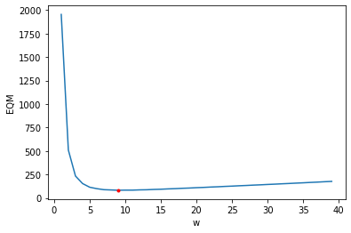
As expected, the MSE change with respect of the filter size. A compromise must be made between the noise reduction and the blurring. We observe that the curve has a minimum, it corresponds to the best choice for \(w\) (in terms of MSE).

The best restoration is obtained for w = 9 and get an MSE = 8.23e+01

Unfortunately, there is no easy way to know a priori the best size of the mean filter just knowing the SNR. The value obtained here depends on the image (try with another image!).

TV denoising

With the noisy image at SNR = 10 dB, we now carry out a denoising by TV regularization.

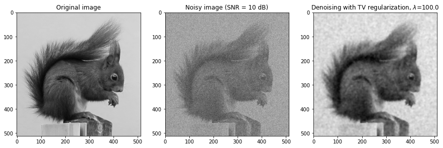
As with the mean filter, we observe that the image is partially denoised (therefore the MSE will be better), but, again, the contours are less sharp, resulting in a degradation of the MSE. As previously, it should exist an optimal value of the regularization parameter \(\lambda\). Let’s see if this denoising technique can surpass the mean filter…

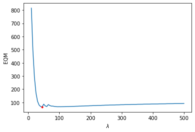
The best restoration is obtained for lambda = 45 and get an MSE = 6.54e+01

The curve has the same behavior as in the case of the mean filter: there is an optimal value of the regularization parameter for which the MSE is the best. Moreover, we notice that the best MSE is lower than the best MSE obtained with the mean filter. So we want to conclude that TV regularization is more efficient than the mean filter! But beware: this conclusion is partial, because it was only obtained on one image with one SNR.

Comparison of the two denoising methods for different SNRs

It is possible to analyze the evolution of the MSE with respect to the noise level by calculating, for several values of SNR, the best parameters for the two methods.

Then we can represent the evolution of the MSE for the two methods:

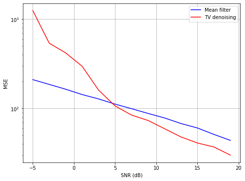
We observe that the MSE decreases with the SNR. The interpretation is easy: the more the noise decreases, the more the image resembles the original image, and therefore denoising is less difficult.

In addition, we observe that:

• for SNRs lower than (approximately) 5 dB, the mean filter is better than TV regularization. This seems surprising since the TV regularization is supposed to be better. However, an SNR lower than 5 dB is extremely low. In fact, neither of the two methods gives a really satisfactory result (see below).

• for images with SNR greater than 5 dB, TV regularization is better.

Let’s see on some examples:

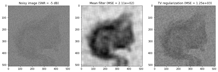
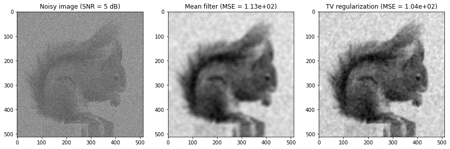
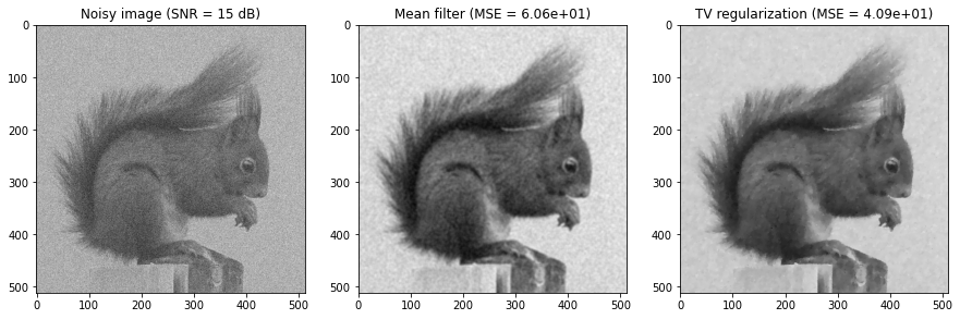
OK, we have the same conclusions as before.

The comparison between the two methods was only carried out on a single image and a single criterion (the MSE). This is undoubtedly a good criterion for comparing two methods, but other criterions exist, such as for example the complexity of the method, the computation time, etc.