Installing and using Python

Python is a modern high-level language with a lot of functions dedicated to image processing. On this page, you will find how to:

• install Python and Jupyter on a computer,

• write notebooks using Jupyter Lab,

• start programming and import specific functions.

Installation

Anaconda is a Python distribution specialized in data science and machine learning. For individual use, it is free and sufficient to perform the image processing exercises. Download and install Anaconda if Python is not already present on your computer. Be careful, choose version 3 (or higher) of Python!

Another similar yet older interface exists: Jupyter Notebook.

Anaconda contains a computational environment for creating Python programs, namely Jupyter Lab. This is an open-source software for interactive computing and it provides a modern interface to write notebooks.

Fig. 110 shows the interface of Jupyter Lab. The interface is quite intuitive, but you can read this page to learn more.

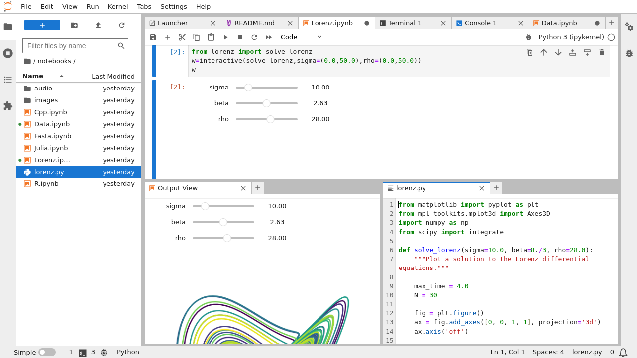
Fig. 110 Jupyter Lab.

Jupyter Lab should be included in the Anaconda installation. But if not, you will find instructions for installing Jupyter Lab here.

Start JupyterLab by typing in a console:

jupyter lab

or

jupyter-lab

Writing a notebook

After installing Python and Jupyter Lab, you are now able to write and execute Python notebooks! A notebook is a file that contains code, but also the results produced by the code (such as numerical values or images) and comments. A notebook is divided into cells which are either “code” cells or “markdown” cells. By pressing Ctrl+Return on a cell, the code of this cell (only this cell!) is executed.

You need specialized software to view and use a notebook, such as Jupyter Lab. A description of this software is given below.

Code cells

By default, cells are expected to contain code. They are divided between an input (with Python instructions) and an output (the result).

For example the following input:

a = 21
b = 42
c = a + b
print("The value is " + str(c))

results in this output:

The value is 63

Markdown cells

You can change a code cell to a markdown cell by choosing Markdown from the drop-down list in the toolbar. Markdown is a very simple language to format text (e.g. writing titles, lists or equations). This will be useful not only for adding notes and comments in your code, but also to write the project report at the end of the course.

For example:

The _convolution_ between **two** images $f$ and $g$ is defined as

$$
  (f*g)(m,n) = \sum_u \sum_v f(u,v) g(u-m,v-n)
$$

results in

The convolution between two images \(f\) and \(g\) is defined as

\[ (f*g)(m,n) = \sum_u \sum_v f(u,v) g(u-m,v-n) \]

Please read this help to learn the markdown syntax.

Writing code

The core of Python does not have functions for scientific computing, so you have to import modules. Generally, we will use the three following modules:

• numpy (version 1.2 or higher), which provides functions for general scientific computing,

• scikit-image (version 0.17 or higher), which is a collection of algorithms for image processing,

• matplotlib (version 3.4 or higher) to display images.

Normally, these packages are installed with Anaconda. If this is not the case, read the documentation given above to get help.

Python modules are imported in your code by using the instruction import.

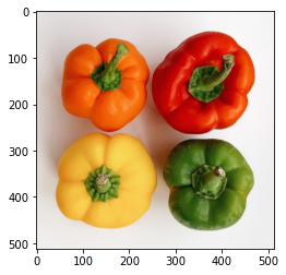
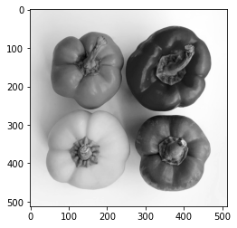
As an example, the following code open an image, convert it to grayscale and display the two versions:

# This is a comment inside the Python code, so it is not executed
# Comments are lines beginning with a #

# Import the sub-module 'io' in the module 'skimage' (a short term for scikit-image),
# and rename it as 'io' (because skimage.io is a bit long and there is no harm in being lazy 😴)
import skimage.io as io

# Import the sub-module 'color' in the module 'skimage', and rename it as 'clr'
import skimage.color as clr

# Import the sub-module 'pyplot' in the module 'matplotlib', and rename it as 'plt'
import matplotlib.pyplot as plt

# The function 'imread' in 'skimage.io' load an image from a filename
f = io.imread("../figs/peppers.png")

# Convert the color image f in grayscale image g
g = clr.rgb2gray(f)

# Display the color image f with the function 'imshow' in 'matplotlib.pyplot'
plt.imshow(f)

# Show the image f
plt.show()

# Display the grayscale image g
plt.imshow(g, cmap="gray")

# Show the image g
plt.show()

For Matlab users

Python, with the use of the module Numpy, is very similar to Matlab. Both work with scripts, and the functions are very similar. However, some major differences exist.

Modules

Python is intended to be a general-purpose programming language. Thus, scientific functions are not included into its core, contrary to Matlab. These functions must be loaded through modules like Matplotlib or Numpy. Fora example, Numpy is loaded with:

import numpy as np

The functions in Numpy are then accessible with np.name_of_the_function.

Vectors and matrices

While Matlab uses round brackets in vectors and matrix, Python uses square brackets. In Matlab, the first element has index 1, while it has index 0 in Python.

Matlab	Python
a(1)	a[0]
B(3,5)	B[2,4]

Semicolon

There is no semicolon (;) at the end of the instructions with Python.

To go further…

To go further, you can read this cheatsheet or read this article on Numpy.