Lab 1

Lab 1#

After completing each exercise, you can refer to the correction. Furthermore, do not hesitate to ask your colleagues and teachers for additional information or to discuss specific topics.

1 Getting started#

Python is a very versatile programming language and can especially be used for scientific programming and image processing. Python’s syntax is very similar to Matlab’s one. Before beginning this lab, you may need to know Installing and using Python. If you use your personal computer, beware of the module version. We will use Jupyter Lab, which runs in a web browser, to write programs. These programs are saved as notebooks.

First, boot your computer on Ubuntu, then open a terminal by typing terminal in the main menu or typing Ctrl + Alt + T.
Start Jupyter by typing in a terminal:
```
jupyter lab
```
or
```
jupyter-lab
```
In Jupyter Lab, open a new Python 3 notebook and rename it from File > Save Notebook As.... A notebook is a file with extension .ipynb.

Now you are ready to write a Python program in the notebook.

In the first cell of the notebook, write
```
40 + 2
```
and type Shift + Return. The code is executed, the result is displayed then a new cell appears below.
Like any programming language, the code is written using variables and functions. A variable stores one (or more) values, whether it is numeric or not. The name of the variable can contain letters, numbers (except the first character) or underscore. Case is important (i.e. a and A are two different variables). Type the instructions below in the second cell:
```
year = 2023
course = "BIP"
```
and type again Shift + Return. Now the value 2023 is stored in the variable year and the character string “BIP” is stored in the variable course.
Modify the previous cell by adding the following statement:
```
print(f"{course} {year}")
```
print is a function and the string in the brackets is an argument. Here, this argument is a character string. The f at the beginning of the string means that it is a formatted string. Type Shift + Return to run again the code.

A notebook is appealing as it is also possible to add text using the markdown language.

Select an empty cell, then click on the drop-down list in the toolbar to select Markdown. Then you can write formatted text. Try to write:

New exercise

Write bold, italic or equations: \(\sqrt{2}\).

This can be useful for inserting titles or keeping comments and notes.

Verify your code in the correction.

2 Display a saved image#

Open a new notebook.
Download the image 4.2.03.tiff (available online) in the same folder as your notebook.
Write in the notebook the following statements to allow the use of the modules skimage.io and matplotlib.pyplot which are renamed io and plt.
```
import skimage.io as io
import matplotlib.pyplot as plt
```
The names io and plt are conventional names, but you can define other terms.

Load :

f = io.imread("4.2.03.tiff")

and display it:

plt.imshow(f)

What are the dimensions (in pixels) of the image?

The conversion of a color image with pixel values \(r\), \(g\), \(b\) to a grayscale image with pixel intensity \(x\) is made through the transformation

\[ x = 0.2125 \, r + 0.7154 \, g + 0.0721 \, b. \]

The coefficients have been obtained by psychovisual studies and guarantee that \(x\in[0,1]\) if \(r,g,b\in[0,1]\).

Convert the color image to grayscale (skimage.color.rgb2gray) then display it.
Print the intensity of the top-left pixel (which is at position \((0,0)\)) by typing g[0,0].
Print the intensities of the five first pixels of the second row by typing g[1,0:5], which extract from g the pixels at row 1 and columns 0 to 4 (the last index is not reached).
Print the intensities of all the pixels in the third row by typing g[2,:], which extract from g the pixels at row 2 and all the columns.

The natural representation of an image is a two-dimensional display where the intensity of the pixels is given by a color. However, an image can also be seen as a three-dimensional curve, opening the way to new interpretations.

Extract a row or a column of pixels from the image, then display this brightness profile as a signal (matplotlib.pyplot.plot). Do you manage to find in this profile the different areas of the image?

3 Display several images#

Open a new notebook.
Download and unzip flowers.zip in the same folder as your notebook.
Create a list with the name of the images contained in flowers.zip. Instead of listing manually the images, you can look for a code on the web, as for example in Stackoverflow.
Print the number of images.
Define a figure with as many subplots as images with matplotlib.pyplot.subplots.
Show each images onto this figure.

4 Create a simple image#

An RGB image is encoded in the form of a three-dimensional array: the first two dimensions are the spatial dimensions of the image, the third corresponds to the bands.

Create the array corresponding to the RGB image \(40 \times 80\) sketched Fig. 109:

Fig. 109 A simple image.#

To do this, create first a black image with the correct dimensions (numpy.zeros generates an array filled with zeros). Then assign the desired value to the elements of the matrix, proceeding band by band, by using for example:
```
f[m1:m2, n1:n2, b] = x
```
This statement assigns the value x to the pixels of the band b located between the rows m1 and m2\(-1\) and the columns n1 and n2\(-1\) (in Python, indices starts at 0).

5 Setting the intensity range#

Display the image hdfs.tiff, corresponding to a part of the sky in the southern hemisphere. You should only observe a single star.
What is the dynamic of this image (i.e. the minimum and maximum values of the intensities)?
Adjust the intensity range with the arguments vmin and vmax of the function matplotlib.pyplot.imshow to observe other objects, most of them being galaxies.
Try another colormap (argument cmap).

6 Segmentation by histogram thresholding#

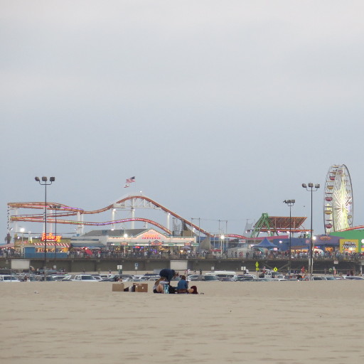
Load the image santamonica.jpg and convert it to grayscale.
Display its histogram with matplotlib.pyplot.hist, after having vectorized the image with numpy.ravel.
Try different bin number and discuss the result: what do you observe?
Choose a suitable threshold to segment the image into two classes. To perform thresholding, the easiest way is to display the image
```
f > threshold
```
where f is the image to threshold and threshold is, well… the threshold value.

7 Contrast enhancement#

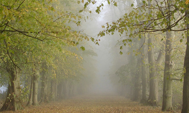
Display the image haze.png, after converting it to grayscale.
Display its histogram. You will notice that the image is not very contrasted: what does that imply on the histogram?
Multiply the image by a positive real: what happens on the image and its histogram? Adjust the intensity range of the image to be the same as the original image.
Perform an histogram equalization (skimage.exposure.equalize_hist). Do you achieve the exercise goal?