Lab 2

Convolution

The image smiley.png will be convolved with several PSF. Before applying the convolutions, you need to convert the image into float (skimage.img_as_float).

Note

It can be very useful for analyzing the results to display the colorbar alongside each image. You can follow the code below (img is the image to show):

import matplotlib.pyplot as plt

plt.figure()
im = plt.imshow(img, "gray")
plt.colorbar(im)
plt.show()

• What does the acronym PSF stand for?

• Compute the convolution between the image and a Gaussian kernel (skimage.filters.gaussian).

• Compute the convolution between the image and the kernel defined by

  \[ h = \begin{pmatrix} 1 & -1 \end{pmatrix}, \]

  by using scipy.ndimage.convolve and initializing \(h\) with numpy.array. We stress that \(h\) being an image, it should be defined as a 2D matrix!

• Compute the convolution between the image and a kernel defined by an array of 30 elements equal to 1/30 (numpy.ones).

Properties of the Fourier transform

• Load the image s1.png and compute its discrete Fourier transform (DFT) with numpy.fft.fft2.

• Show the DFT of the image with low frequencies at the center (numpy.fft.fftshift). The magnitude and angle are obtained with numpy.absolute and numpy.angle.

You wrote a code that computes and displays the DFT of the first image. Instead of repeating five times this code, a good practice is to insert the code into a for loop which iterates over a list of the images.

• Repeat the same operations with images s2.png, s3.png, s4.png, and s5.png. Analyse the specificities of the images: what can you say about the DFT?

Filtering aliasing

Aliasing (french: crénelage) is a phenomenon that occurs when the image is poorly sampled. It can be avoided by applying an anti-aliasing filter (french: filtre anti-repliement) before sampling.

Warning

Do not display the images in the notebook in this exercise! Jupyter Lab and Matplotlib can create aliasing on display. Instead, save the images with skimage.io.imsave and look at them with an external viewer, by taking care of using a 100% zoom.

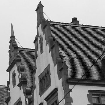
• Load and display the image roof.jpg. Then, downsample it (without an anti-aliasing filter) by a factor of three by taking one pixel out of three in the two spatial dimensions, which can be done with the instruction

  f[::3,::3]
  

  How does the phenomenon of aliasing appear visually?

• Now, apply a Gaussian filter (skimage.filters.gaussian) to the original image before downsampling. Adjust the filter parameter to minimize aliasing. Is the aliasing still visible?

• Lastly, replace the Gaussian filter with an ideal low-pass filter, which completely eliminates frequencies above the cutoff frequency without modifying the frequencies below. The process is:

  1. Compute the DFT of the image,

  2. Define the ideal filter as a zero image with a square of 1 in the Fourier domain,

  3. Multiply the DFT of the image with the filter (this is equivalent to a convolution in the spatial domain),

  4. Compute the inverse DFT of the result (and keep only the real part).

  The code below generates a binary square mask of the same size as the image X:

  Mask = np.zeros(X.shape)
  Mask[a:b,c:d] = 1
  

  Choose correctly the coordinates a, b, c and d to conserve the low frequencies, which are located at the center in the DFT (after applying numpy.fft.fftshift).

  The ideal filter may be defined in the same way as in the exercise 4 Create a simple image: use the function numpy.zeros and the indexing f[m1:m2,n1:n2]=x. Choose the cutoff frequency appropriately to reduce aliasing without altering the image. Is the aliasing still visible?