5 Setting the intensity range

Display the image

Load and display the image:

f = io.imread("hdfs.tiff")
plt.figure(figsize=(6,6))
plt.imshow(f, cmap="gray")
plt.show()

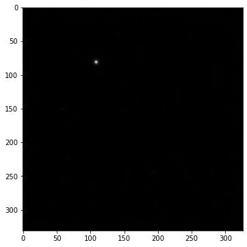
This image corresponds to a portion of the sky in the southern hemisphere called the Hubble Deep Field South. It was acquired by the MUSE sensor installed on the VLT in Chile. It is obtained by averaging around 4000 bands of the original image: we speak of a hyperspectral image (source: Bacon et al., “The MUSE 3D view of the Hubble Deep Field South”, Astronomy & Astrophysics, 2015).

Sketch the histogram

Although only a small star can be seen, there are many other astronommimcal objects. Since these objects are very distant, they are very faint. In astronomy, as in many other science fields, the pixel intensity is not limited to 256 values. In this case, the intensities lie over the range given below:

print("Mininmal intensity: %d" % f.min())
print("Maximal intensity: %d" % f.max())

Mininmal intensity: 625722
Maximal intensity: 628454834

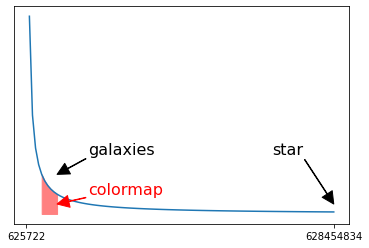
Here is a sketch of what should be the histogram. Most of the pixels are very dark hence the peak at the minimum intensities. In this peak (but not at the minimum value) lie the galaxies. Thus, the colormap is expected to be somewhere around the red area.

Choose a better colormap

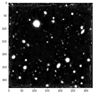
Therefore, to observe the other objects, we will adjust the colormap so that the gray levels will lie between vmin and vmax. Intensities less than vmin will be displayed in black, intensities greater than vmax will be displayed in white, and intensities in between will be displayed with the different levels or gray. It’s up to you to find these values to get an image like the one below, where other stars and galaxies are clearly visible (and the brightest star is saturated).

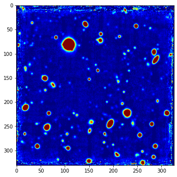
Another possibility is to use colors to increase the dynamics of the intensities observed. The jet colormap is used in the example below, with the the same vmin and vmax as before. We observe a few more objects.