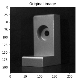
Sobel and Canny detectors

Sobel and Canny detectors#

The objectives of this exercise are to:

detect edges using Sobel and Canny detectors
understand the influence of the parameters of these methods
compare these methods in terms of computation time

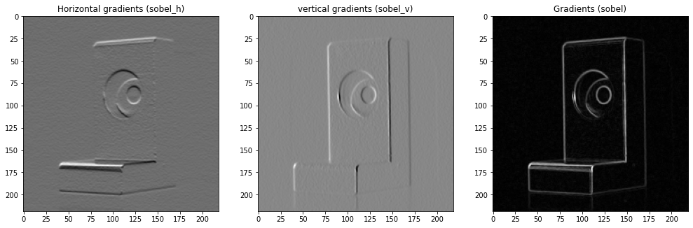
../_images/01411dfda0cfab22b38eaaccc5f92175bd468fb81f47ab9466d6bff1f3a5315e.png

Sobel detector#

The Sobel detector performs a convolution of the image by two filters, each allowing to obtain the gradient of the image in the two dimensions. These two gradients can be merged to result in the right image (how are they merged?).

../_images/c4f4ddcf309e8662aea96f4befe412eac7ae486a6e5f2e74cf45236265855075.png

The gradient image can be thresholded to identify major contours. The results for three threshold values are given below.

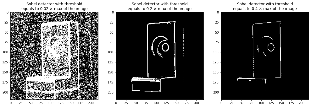
../_images/4d99c502fd48dda4012e2ae92119d9172c26ff070ec901d21446be8a62eb1fc1.png

We note that the higher the threshold, the fewer contours detected (there are fewer white pixels). This is because fewer pixels have a gradient greater than the threshold, and therefore will be considered as edges.
If the threshold is too low, then edges are detected almost everywhere. In particular, the background of the image being (slightly) noisy, edges can be detected there.
On the contrary, if the threshold is too high, then there are a lot of non-detections even though there are hardly any false alarms left.
In addition, even by setting the threshold high enough, some edges are still wide: they have a width of several pixels, which implies that the edge, although detected, is not positioned with precision.

Canny detector#

Canny detector is more complex than a simple filtering. It includes in particular a thresholding by hysteresis, i.e. a decision based on two thresholds \(T_{low}\) and \(T_{high}\):

the pixels of intensity lower than \(T_{low}\) will not be considered as edges,
pixels with an intensity greater than \(T_{high}\) will be considered as edges,
pixels with an intensity between \(T_{low}\) and \(T_{high}\) will be detected as edges if and only if they are neighbors of pixels whic are edges.

Influence of the Gaussian standard deviation (`sigma`)#

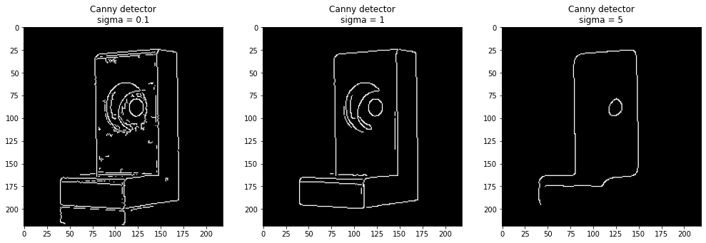
../_images/cea2f38d25d57883ed01885f48a7a6e6f9f92180e82d278d20dc9d1d2a526cd6.png

We observe that if sigma increases, then the number of edges detected is lower. This can be explained by the fact that the first step of the Canny detector is a filtering of the image by a Gaussian (with standard deviation sigma) to reduce the noise. In consequence, the image is more blurry and therefore the edges are less marked: they are therefore more difficult to detect.

Influence of \(T_{low}\) (`low_threshold`)#

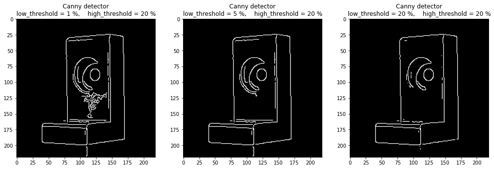
../_images/e17c89efeefb0e5b04a38336f7fb3412340be40e70b6fe5040fcbe70d0ea934e.png

When the lower threshold increases, the number of detected edges decreases, since there are fewer pixels whose gradient value is greater than the lower threshold.

Influence of \(T_{high}\) (`high_threshold`)#

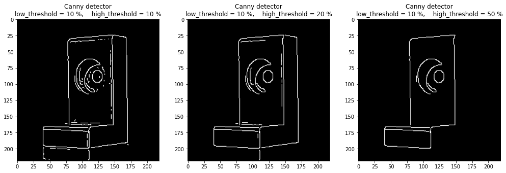
../_images/119f3e052882b9ce8a9cfd509ddb686879a44e11323404e62af6ac2b1cc4720f.png

As before, the more the higher threshold increases, the fewer edges are detected.

In conclusion, we observe that the number of detected edges decreases with the value of the thresholds, as for the Sobel detector. Besides, the Canny detector produces fine and mostly continuous contours: detection is therefore clearer and more precise.

Comparison of the two methods in terms of computation time#

One of the steps of the Canny detector is to apply a Sobel filter. So the Canny detector is expected to be slower than the Sobel detector. We measure the time required for each method to detect the edges of the image.

For practical reasons, depending especially on the computer used for the test, the results are not perfectly reproducible: if you run the comparison twice, the computation times will differ slightly. Therefore, it is advised to measure the computation times over many simulations (100 below).

I = 100           # Number of simulations
total_sobel = 0   # Total time for the I simulations for the Sobel detector
total_canny = 0   # Total time for the I simulations for the Canny detector

for i in range(I):
    
    # Computation time for the Sobel detector
    tic = time.time()
    y = sobel(x)
    z = y > 0.5*y.max() # Don't forget to take thresholding into account!
    tac = time.time()
    time_sobel = tac-tic
    total_sobel += time_sobel
    
    # Computation time for the Canny detector
    tic = time.time()
    z = canny(x)
    tac = time.time()
    time_canny = tac-tic
    total_canny += time_canny
    
    # Display the computation time of the two methods (for the first 10 simulations only)
    if i<10:
        print(f"Sobel : {time_sobel*1e3:.3f} ms     Canny : {time_canny*1e3:.3f} ms")
    elif i==10:
        print("etc.")
    
print(f"\nCanny detector is, about {total_canny/total_sobel:.0f} times slower than Sobel detector.")

Sobel : 2.935 ms     Canny : 16.135 ms
Sobel : 3.383 ms     Canny : 18.684 ms
Sobel : 3.484 ms     Canny : 16.753 ms
Sobel : 3.050 ms     Canny : 14.943 ms
Sobel : 2.366 ms     Canny : 14.675 ms
Sobel : 2.423 ms     Canny : 14.041 ms
Sobel : 2.345 ms     Canny : 13.976 ms
Sobel : 2.288 ms     Canny : 13.934 ms
Sobel : 2.286 ms     Canny : 13.968 ms
Sobel : 2.297 ms     Canny : 14.032 ms
etc.

Canny detector is, about 6 times slower than Sobel detector.

We were right: Canny detector is slower than Sobel detector. However, the computation time remains very acceptable for images of classic size (around 15 ms), so the time difference between the two methods is not detrimental in the majority of applications.

Sobel and Canny detectors

Contents