Human vision
Figure 1 shows a simplified cross section of the human eye.
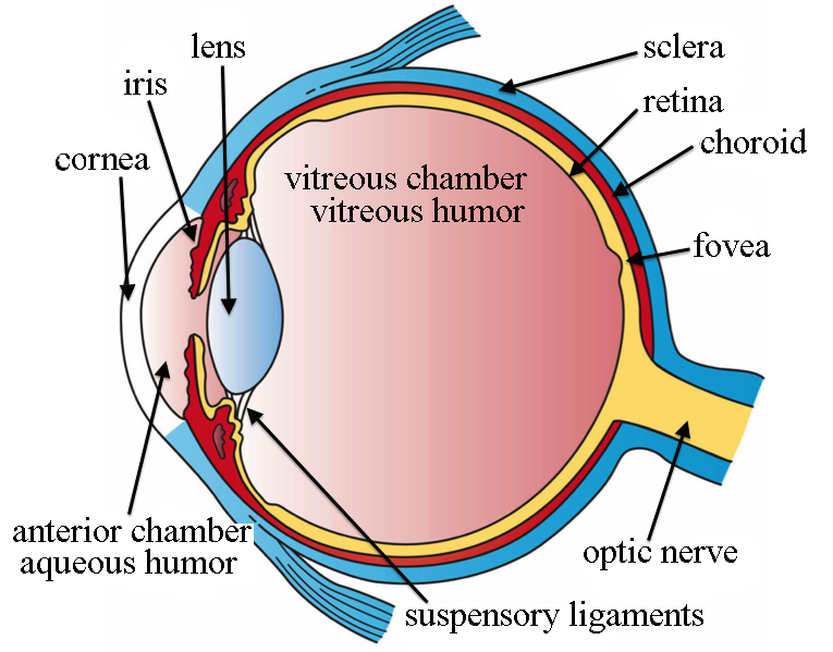
Figure 1:Simplified diagram of the human eye.
The eye is basically composed of:
the cornea (French: cornée), a transparent tissue that covers the surface of the eye,
the lens (French: cristallin), a second transparent tissue that refracts light onto the retina by changing its shape,
the retina (French: rétine) which lines the inside of the posterior portion of the eye. The light from an object is imaged on the retina when the eye is properly focused.
The human eye’s retina contains two kinds of receptors. The rods (French: bâtonnets) provide an overall picture of the field of view and are sensitive to low levels of illumination. The cones (French: cônes) allow color vision. There are three types of cones which are sensitive to short (S), medium (M) and long (L) wavelength of the visible light (see Figure 2). Basically, they are sensitive to blue, green and red light. Rods and cones are connected to the brain by nerves, which proceeds to the image analysis.
Figure 2:Responsivity of the three kinds of cones, compared to electromagnetic spectrum.
Image acquisition
The principal phenomenon at the origin of the acquisition of an image is the electromagnetic spectrum. Images based on radiation from the electromagnetic spectrum are the most familiar, especially images from visible light, as photography. Other images based on the electromagnetic spectrum include radiofrequency (radioastronomy, MRI), microwaves (radar imaging), infrared wavelengths (thermography), X-rays (medical, astronomical or industrial imaging) and even gamma rays (nuclear medicine, astronomical observations).
In addition to electromagnetic imaging, various other modalities are also employed. These modalities include acoustic imaging (by using infrasound in geological exploration or ultrasound for echography), electron microscopy, and synthetic (computer-generated) imaging.
Examples of image modalities
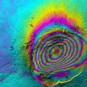
Interferometry.
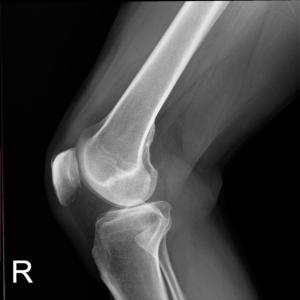
Radiograph of the right knee.
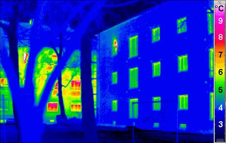
Thermogram of a passive building, with traditional building in the background.
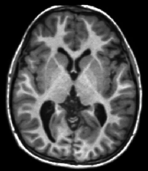
MRI of the brain (axial section) showing white matter and grey matter folds.
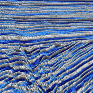
Seismic reflection image.

Image of pollen grains taken on a electron microscope.
In the following, we focus mainly on electromagnetic imaging, especially through visible light.
Sensor (electromagnetic imaging)
A photodiode is the most common and basic sensor for image acquisition with visible light. It is constructed of silicon materials so that its output voltage is proportional to incoming light.
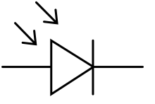
Figure 9:Electronic symbol of a photodiode.
To acquire a 2D digital image, the typical system involves using a matrix of single sensors. Two technologies coexist.
The prevailing technology to read the output voltage of each single sensor is the CMOS (complementary metal oxide semi-conductor) approach: each single sensor is coupled with its own analog-to-digital conversion circuit. This simple counting process makes CMOS technology cheap and low energy. However, it may be less sensitive and can produce distortions in case of rapid movements in the field of view.
On the other hand, the CCD (charge coupled device) approach has declined since the 2010s. The fundamental idea of the CCD is the use of a unique conversion circuit. The potential of each sensor is moved pixel by pixel: the potentials are shifted by one column, then those at the last column are counted by a unique circuit. CCD is progressively disappearing because of several reasons: moving potentials is not instantaneous and consumes energy, and it sometimes creates undesirable side effects, such as blooming.
To reproduce human color vision, the acquisition mimics the three kind of cones by using three kind of filters in front of the sensors. Then, three images are actually acquired, corresponding to the short (blue), medium (green) and long (red) wavelengths. The Bayer filter (Figure 10) is the widely used technique for generating color images. It is a mosaic of red, green and blue filters on a square grid of photosensors. Note that the filter pattern is half green, one quarter red and one quarter blue. The reason for having twice green filter than the other colors is because the human vision is naturally more sensitive to green light.
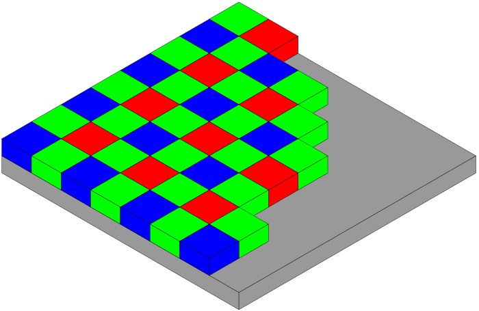
Figure 10:The Bayer filter on an image sensor.
Sampling and quantization
The final step of digital image formation is digitization, which is both the sampling and quantization of the observed scene.
Sampling
Sampling corresponds to mapping a continuous scene onto a discrete grid. This is naturally done by the matrix of pixels. Sampling a continuous image leads to a loss of information. Intuitively, it is clear that sampling reduces resolution and that fine structures will be lost. Thus the number of pixels on the sensor, directly related to the sampling, is crucial (see Figure 11).

Figure 11:Images made of black and white squares of different sizes. The results show significant aliasing for squares of size 0.8 and 0.12 pixels. Note that the right image looks like a “normal” image.
Besides, distortions also occur when resizing an image with fine structures, as seen in Figure 12.

Figure 12:Me with my favourite moiré shirt. Left: image of size 1000×1000, right: image of size 595×595.
This kind of distortion is called aliasing. It is also called moiré effect in images with pediodic or nearly periodic components. To avoid aliasing, one has to satisfy the sampling theorem which states that a continuous scene can be sampled with no error if the sampling intervals are
where and are the sampling intervals in the two directions (i.e. the distance between two consecutive samples) and and are the periods of the finest structures in the image.
In practice, one prefers to put an optical low-pass filter before the sensor to vanish the high frequencies responsible for aliasing, that is to increase and such that the sampling theorem is satisfied.
Quantization
Quantization corresponds to mapping the continuous light intensities to a finite set of numbers. Typically, image are quantized into 256 gray values; then, each pixel then occupies one byte (8 bits). The reason for assigning 256 gray values to each pixel is not only because it is well adapted to the architecture of computers, but also because it is good enough to give humans the illusion of a continuous change in gray values.

name: F:digital-images:quantization width: 100% Quantization of the same image with (from left to right) 256, 16, 4, and 2 gray levels.
However, quantization naturally introduces errors on the intensities. If the quantization levels are equally spaced with a distance and all gray values are equally probable, the standard deviation of the quantification error is lower than [Jähne 2005, p. 243]. For most common applications, the error is sufficiently low to be acceptable. But some applications, such as medical imaging or astronomy, require a finer resolution and, in consequence, use more than 256 gray levels.
Distortions
In addition to the moiré effect and quantization noise, other distortions can affect the image acquisition. The two main distortions are noise and blurring.
Noise
Noise introduces erroneous intensities in the digital image. Sources of noise are multiple, from electronic noise due to the imaging system itself to the acquisition conditions (low-light-level for example). The main noise models are desribed in C:denoising:noise-sources: Gaussian noise, Poisson noise and salt-and-pepper noise. In specific imaging systems, other noise can be encountered. For example, in radar imaging systems the noise is considered to be multiplicative and is called speckle noise.

Figure 14:Noise on a photograph taken in a dark room (this noise is called “dark current”).
Point spread function
Despite the high quality of an imaging system, a point in the observed scene is not imaged onto a point in the image space, but onto a more or less extended area with varying intensities. The function that describes the imaging of a point is an essential feature of the imaging system and is called the point spread function or PSF (French: fonction d’étalement du point). Generally, the PSF is assumed to be independent of the position. Then, the imaging system can be treated as a linear shift-invariant system, which is mathematically described as a convolution (see the dedicated chapter). Sometimes, an imaging system is described not by its PSF but by its Fourier transform, and it is called optical transfer function, or OTF (French: fonction de transfert optique).

Figure 15:Example of blur (parliament of Budapest).