The (2D) Fourier transform is a very classical tool in image processing. It is the extension of the Fourier transform for signals which decomposes a signal into a sum of complex oscillations (actually, complex exponentials). In image processing, the Fourier transform decomposes an image into a sum of oscillations with different frequencies, phase and orientation.
So, the Fourier transform gives information about the frequency content of the image, i.e. how the intensities in the image are distributed through different frequencies. Figure 1 shows the decomposition of a synthetic image into oscillations. In this toy-example, the image is simple enough to be decomposed by using only three oscillations. We will see further that usual images need much more oscillations.
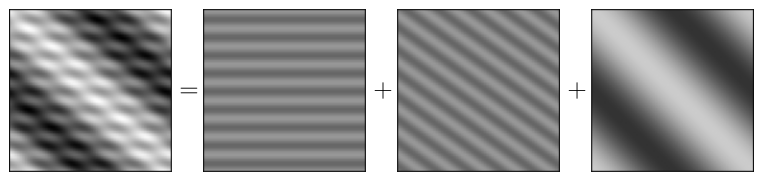
Figure 1:A synthetic image and the three oscillations (frequencies) that compose the image. The third oscillation (on the right) is of lower frequency than the first two oscillations, because the alternation of black and white pixel is smoother than on the first oscillations.
Direct Fourier transform
The discrete Fourier transform (DFT) of an image of size is an image of same size defined as:
In the sequel, we note the DFT so that .
Note that the definition of the Fourier transform uses a complex exponential. In consequence, the DFT of an image is possibly complex, so it cannot be displayed with a single image. That is why we will show the amplitude (modulus) and phase (argument) of the DFT separately, as in Figure 2.
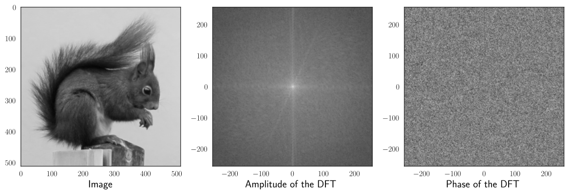
Figure 2:DFT of the squirrel. The amplitude is shown with a logarithmic scale to distinguish clearly the details (an histogram transformation has been applied).
The amplitude and phase represent the distribution of energy in the frequency plane. The intensities of the low frequencies are located in the center of the image, and the intensities of the high frequencies near the boundaries.
In the figure above, the gray background behind the squirrel “contains” mainly low frequencies because the intensities of the pixels slowly evolve from one pixel to another. On the contrary, high frequencies are needed in the tail to show the rapid alternation between the hair and the background.
Inverse Fourier transform
The inverse discrete Fourier transform computes the original image from its Fourier transform:
It is denoted below.
Example of simple Fourier transforms
In the examples below, the image (and their FFT) are 16×16 grayscale images.
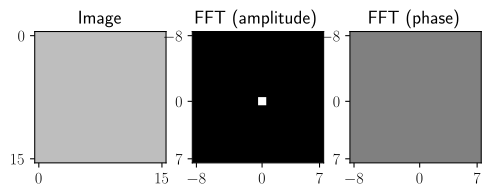
On this example, only the pixel at frequency (0,0) in the Fourier domain is non zero. Because an oscillation with frequency 0 does not oscillate, the image is constant.
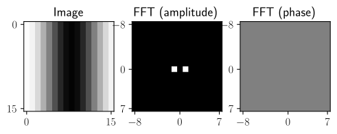
Two pixels in the Fourier domain are non zero. Because they are at frequency 1 along the x-axis, the image is a sinusoid along the x-axis.
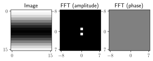
Same example as above along the y-axis: the image is then a sinusoid along the y-axis.
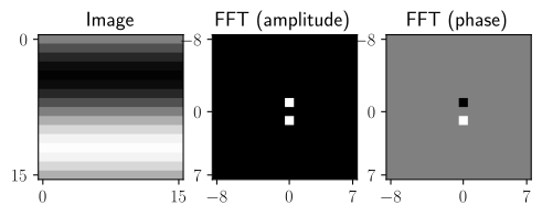
Same example as above with a change in the phase. Therefore, the sinusoid is translated in the spatial domain.
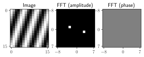
Here, there is a oscillations both in x and y, with high frequency in x and low frequency in y.
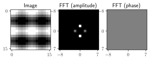
Two waves with are superimposed, both with the same frequency and phase but different orientations and amplitudes.
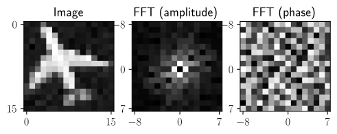
By combining oscillations at appropriate frequencies, phase and amplitudes, it is possible to generate a specific image (here, the mean of the image is set to 0).
Properties
The DFT is linear:
The convolution of two images is equivalent to the multiplication of the DFT of the images, provided that the convolution is circular (wrapping hypothesis on the edges):
The DFT is separable: it can be obtained by computing a 1D DFT on the rows, then a 1D DFT on the columns.
The DFT is periodic with periods and ():
A translation on the image implies a phase shift on the DFT:
A rotation on the image implies the same rotation on the DFT.