Definition
Many image processing results come from a modification of one pixel with respect to its neighbors. This is the case, for example, for blurring.
When this modification is similar in the entire image , it can be mathematically defined using a second image which defines the neighbor relationships. This results in a third image . This is the so-called convolution [Jähne 2005, section 4] and it is denoted with :
Intuitively, the convolution “spreads” each pixel in following and proportionally to the intensity . Figure 1 gives an example of the computing of a particular pixel.
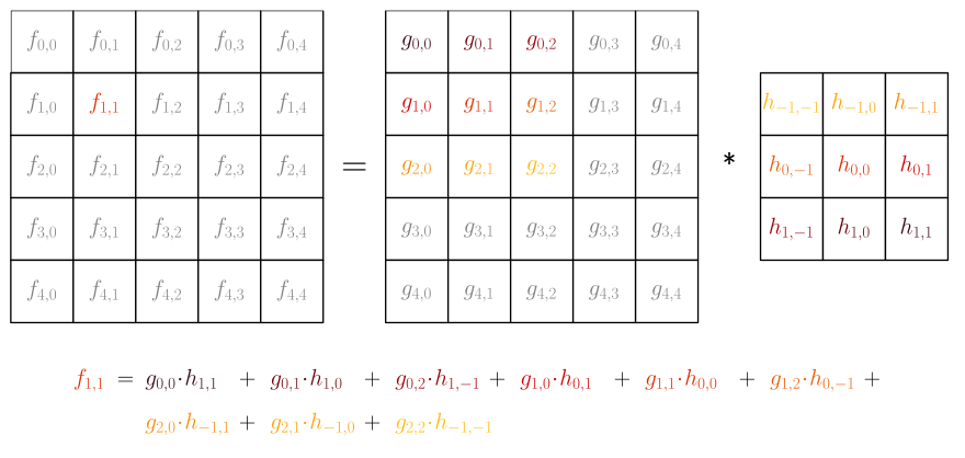
Figure 1:Example for computing the pixel (1,1) of . Note that the pixel (0,0) in the PSF is the one at the center.
For the sake of simplicity, the image is often:
of odd size (, , ...);
centered, i.e. the pixel with coordinates is at the center of the image .
The image is called by different names, depending on the context: filter, mask, kernel, window, pattern or point spread function (PSF).
Some convolution examples are shown above.
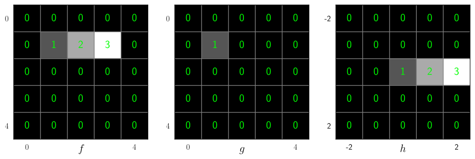
Figure 2:The image to the left is the convolution of the other two images.
Since has only three non-zero pixels, then the convolution formula has only three non-zero terms, and reads:
Then:
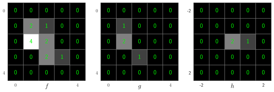
Figure 3:The image to the left is the convolution of the other two images.
Another example which is simple enough to verify by calculating the convolution formula by hand.
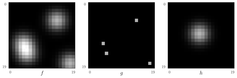
Figure 4:The image to the left is the convolution of the other two images.
is an image composed of only four non-zero pixels. is a blurry spot. The convolution of by clearly shows the “spreading” effect: the result corresponds to each of the four pixels of , at the same position as on , spreading according to the pattern shown on . Notice that the “spreading” of the two nearby pixels adds up, thus giving a very bright area.
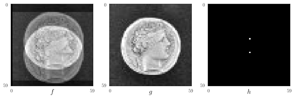
Figure 5:The image to the left is the convolution of the other two images.
Here, each pixel of appears twice in : the result then becomes the image which also appears twice. Another interpretation can be done: the result corresponds to the two unique pixels of which spread while reproducing the pattern .
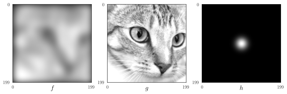
Figure 6:The image to the left is the convolution of the other two images.
is an image made up of pixels of different intensities. Each of these pixels spreads over the result following the pattern . This results in a blurry image. We will see in Filtering that we have applied here a low pass filter on the image .
Properties
As a mathematical operation, the convolution has several properties.
The neutral element of convolution is an image filled with zeros but the pixel at the center equals 1.
The convolution is commutative: .
The convolution is distributive with respect to the addition: .
The convolution is bilinear: (with ).
The convolution is associative: .
Boundaries effects
The convolution formula is not defined on the boundaries of the image: as an example, computing in Figure 1 requires the value of which is not defined.
Therefore, one has to make assumptions about the pixel values outside the image. Figure 7 shows an image with some possibilities to consider the external pixels, and Figure 8 shows the convolution of these images by a Gaussian.
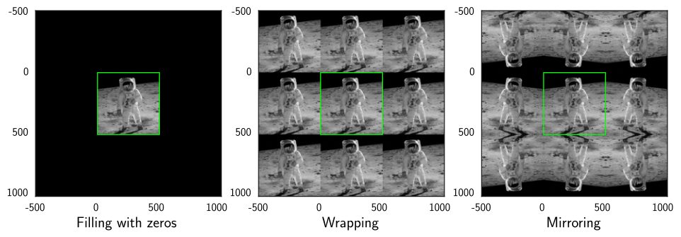
Figure 7:Several ways to assume the pixels outside the image. The image is delimited by the green edge.
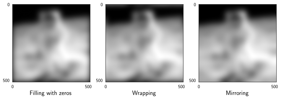
Figure 8:Results of the convolution with the same image.
One can see on the Figure 8 that the three convolutions are basically identical: only the pixels near the boundaries may be different (darker or brighter on this example). Anyway, there is no perfect choice to set the pixels outside the image, and each choice yields some errors. Also, the best thing is to ensure when acquiring the image that the objects of interest are far from the edges
At last, note that the wrapping hypothesis yields a circular convolution. This is also the result given by a multiplication in the Fourier domain (see Fourier transform).
Separable Convolution
A separable convolution is when the convolution kernel can be written as the convolution of two 1D filters (say and ) defined along the two axes. Let’s give an example.
If the PSF can reads
then
Thus, the convolution of an image by a separable filter can be calculated by first computing the convolution of with , then the convolution of the former result with (or the reverse):
The convolution separability saves computation time because the computation of two 1D convolutions requires less operations than the computation of a 2D convolution.
Proof
Consider two images and of size .
On the one side, the computation of one pixel by using the 2D convolution needs multiplications and additions. Therefore, computing the convoluted image needs operations.
On the other side, each element of a 1D convolution along one column needs multiplications and additions. Similarly, each element of a 1D convolution along one row needs multiplications and additions. Therefore, computing the convoluted image needs operations.
It is easy to see that operations, highlighting the efficiency of the separability.