SIFT - Basics of Image Processing

The scale-invariant feature transform (SIFT) algorithm was proposed by Lowe in 1999 [Lowe 1999] to detect specific pixels in images and to match them between two images by using the descriptors that characterize them. SIFT is still one of the most popular feature detectors today because the algorithm is robust to translation, scaling, rotation, partial occlusion or illumination changes. Applications include object recognition, video tracking, robotic navigation, image composition (stitching), etc.

The 6 stages in SIFT are the following and they are described in the next sections:

a scale space with Gaussian kernel is computed so as to get a collection of images with different blur level and resolution,
at each resolution, a few difference-of-Gaussian are computed : they are the data to find the following keypoints,
pixels with high intensity variation in the scale space are detected: they are the so-called keypoints,
the main orientation gradient is determined in a local window centered on the keypoints,
descriptors (vectors with 128 values) are computed for each keypoints,
finally a matching is possible between keypoints and their descriptors of two images.

Scale-space representation¶

A (discrete) scale-space representation is a family of images with increasing blur levels and decreasing resolution. SIFT uses a a Gaussian kernel, so the image at each level $L$ is getting by:

convolving the image $f(x,y)$ by a Gaussian $g(x,y,\sigma_L) = \frac{1}{2\pi\sigma_L^2} e^{-(x^2+y^2)/2\sigma_L^2}$ to produce a blurred image

\ell(x,y,\sigma_L) = f(x,y) * g(x,y,\sigma_L)

downsampling the blurred image $\ell(x,y,\sigma_L)$ by a factor 2 using bilinear interpolation.

In practice, the blurred images $\ell(x,y,\sigma_L)$ can be efficiently computed by applying two passes of a 1D Gaussian function in the horizontal and vertical directions (the 2D Gaussian function is separable).

The series of blurred and downsampled images produces a pyramid representation (see Figure 1) and each level is called an octave.

Figure 1:Scale space representation [Wikipedia].

Difference-of-Gaussian at each scale¶

At each octave $o$ of the scale space, $K$ blurred images are produced:

\ell(x,y,\sigma_{L,k}) = f(x,y) * g(x,y,\sigma_{L,k})

where $\sigma_{L,k}$ ( $k\in\{1,\dots,K\}$ ) is the parameter of the Gaussian kernel and depends on the level $L$ , the parameter $\sigma_L$ and the number of blurred image at level $L$ (see [Lowe 2004] for details).

Then, we compute the difference ( $k>0$ ):

\begin{align*} D(x,y,\sigma_{L,k}) &= \ell(x,y,k\sigma_{L,k}) - \ell(x,y,\sigma_{L,k}) \\ &= f(x,y) * \big( g(x,y,k\sigma_{L,k}) - g(x,y,\sigma_{L,k}) \big) \end{align*}

where $(g(x,y,k\sigma_{L,k}) - g(x,y,\sigma_{L,k}))$ is called the difference-of-Gaussian (DoG). It can be seen that the DoG acts as a bandpass filter.

Figure 2:Scale space and DoG at each octave and for each couple of blurred images [Lowe 2004].

Keypoint detection¶

The keypoints are pixels in the image that are invariant to scale and orientation. To detect keypoints, each pixel in a blurred image (at each octave and scale) is compared to its 8 neighbors in the current image and 9 neighbors in the scale above and below (see Fig. X). This gives a total of 26 neighbors.

Extrema of the DoG images are detected by comparing a pixel (marked with X)
to its neighbors (marked with circles) at the current and adjacent scales
[Lowe 2004]. — Figure 3:Extrema of the DoG images are detected by comparing a pixel (marked with X) to its neighbors (marked with circles) at the current and adjacent scales [Lowe 2004].

The pixel is then considered as a keypoint if and only if it is an extremum in its neighboring, that is it is greater or smaller than all of its neighbors. Note that some detected keypoints are discarded if they are low contrasted or if they lie on an edge (because their localization cannot be precise enough along the edge).

Example of DoG scale-space on an image (left).
[Rey Otero 2014]. — Figure 4:Example of DoG scale-space on an image (left). [Rey Otero 2014].

Keypoints orientations¶

Each remaining keypoint is assigned to an orientation so that the descriptors are invariant to rotation.

In order to make the orientation as stable as possible against lighting or contrast changes, the orientation is not the gradient angle but is determined from histogram of oriented gradient (HOG). HOG is simply the histogram of the gradient angles in a window around the keypoint: each pixel in the window contributes to the histogram by adding a value equal to the gradient magnitude to the (nearest) bin corresponding to the gradient orientation (Figure 5).

HoG on a 160×160 image.
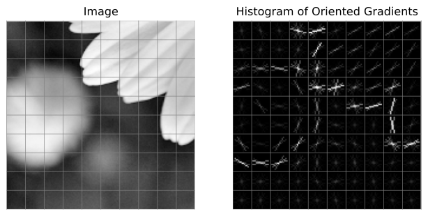
Each window is of size 16×16. — Figure 5:HoG on a 160×160 image. Each window is of size 16×16.

In SIFT, the histogram has 36 bins covering the 360 degree range of rotations. The orientation to assign to the keypoint is determined by the highest peak in the histogram.

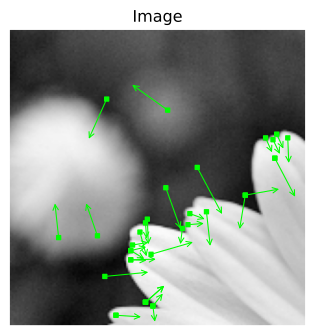
Figure 6:Keypoints and their orientation.

Keypoints descriptors¶

A descriptors is, generally, a list of numerical values that characterize the keypoint. This stage consists in computing a descriptor for the local region around each keypoint, so that the desciptor is as invariant as possible to remaining variations, such as change in illumination or 3D viewpoint.

Again, the magnitude and angle of the gradient is used to define the desciptor. So, a 16×16 window centered on the keypoint is defined, furthermore it is oriented relative to the keypoint orientation in order to be invariant in rotation (Figure 7).

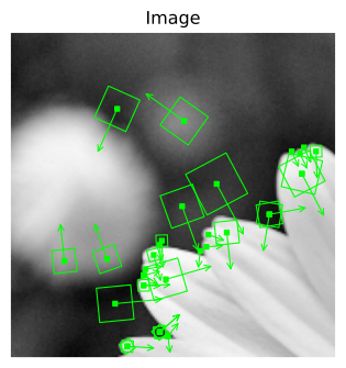
Figure 7:Keypoints, their orientation, and their windows where an HoG is computed.

The 16×16 window is divided into 16 cells where an HoG is computer with 8 orientation bins in each. The descriptor is the vector containing the values of all the orientation histogram entries, therefore, it continas 16×8 = 128 element features.

Matching¶

The final stage of SIFT is to find matching between the descriptors of one image with the descriptors of a second image. To do that, the descriptors are considered as points in a 128-dimensional space. The goal is to find the lowest Eclidean distance between the points The descriptor $d_i^1$ of image 1 is paired to the descriptor $d_j^2$ of image 2 that minimizes the Euclidean distance between descriptors. A pair is considered reliable only if its distance is below a certain threshold, otherwise it is discarded.

This matching problem considered the pairing of, typically, thousands of descriptors in a high dimensional space: it is known to have high complexity if an exact solution is required. Instead, a modification of the k-d tree algorithm called the best-bin-first search method is used to identify the nearest neighbors with high probability, using only a limited amount of computation.

Figure 8 shows an example of matching.

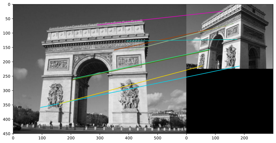
Figure 8:Example of matching on the main paired keypoints.

Alternatives to SIFT¶

SURF (Speeded-Up Robust Features) [Bay 2006] accelerates SIFT so it is more suitable for real-time applications. The main differences with SIFT are the following:

Integral images are used to deal with convolutions. An integral image $I$ represents the sum of all pixels in the input image $f$ that are in the rectangular region formed by the origin and the pixel in $I$ :
$I(x,y) = \sum_{m=0}^{x} \sum_{n=0}^{y} f(m,n).$
DoG approximates a second derivative (or Laplacian, which is actually the trace of the Hessian matrix). SURF replaces DoG by a fast approximation of the Hessian matrix.
The orientation of the keypoints are determinated with Haar wavelets, which are a series of binary masks with rectangular regions.
Other simplifications allows to simplify the different stages of the SIFT algorithm to the essential. For instance, SURF produces a 64-dimensional descriptor, which is more compact and faster to compute than SIFT descriptor.

ORB (Orientated FAST and Robust BRIEF) [Rublee 2011] is considered to be roughly 10 times faster than SURF, while performing as well in many situations.