An edge (French: contour) in an image is the frontier that delimits two objects. Therefore, edge detection is useful for identifying or measuring objects, or segmenting the image.
The advantage of using the derivatives
Edges are characterized by a rapid variation in the intensity of the pixels. Figure 1 represents the brightness profile along a horizontal line in the image. One clearly sees that the outline of the industrial piece shows a sudden decrease in the brightness of the pixels.
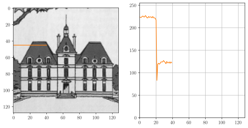
Figure 1:An image and the luminosity profile on it.
From this example, it appears that derivation is an efficient tool for highlighting the edges: an edge can be detected by analyzing the first derivative of the intensity profile, taken perpendicular to the edge. Similarly, an edge can be detected by determining the zero-crossing of the second derivative.
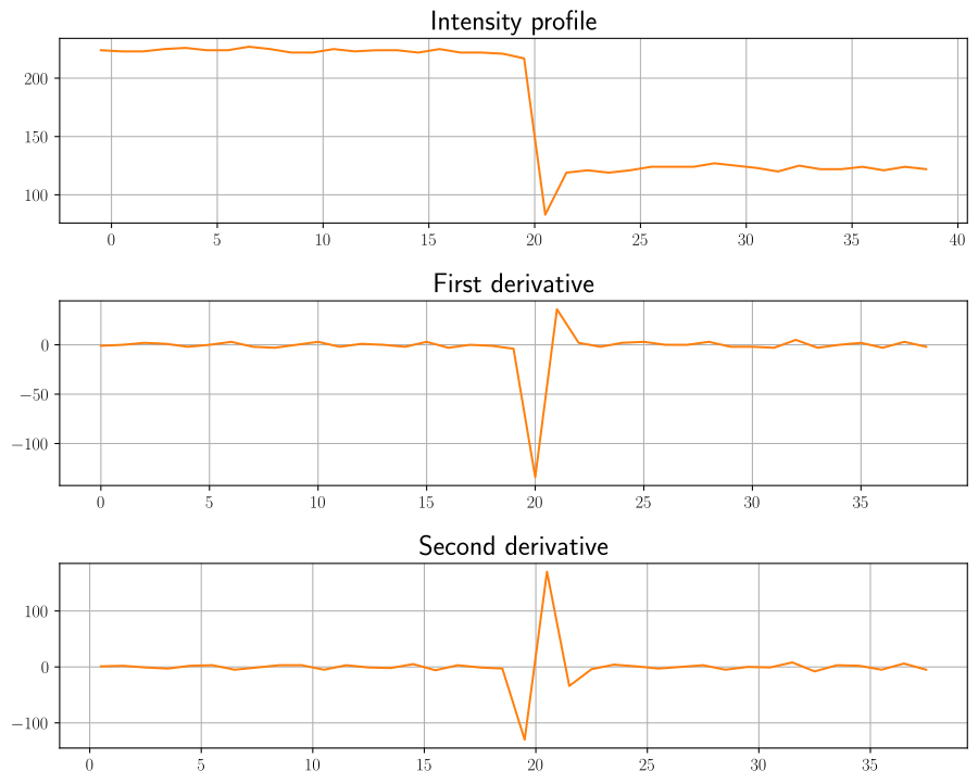
Because an image depends on two dimensions, the derivatives must be calculated according to the two axes. In addition, the derivatives are discrete differences in the case of digital images. Then, the first derivative of a digital image are defined as:
The first derivatives are gathered in the so-called “gradient” (French: gradient) defined as:
In the same way, the second derivative, called “Laplacian” (French: laplacien), is defined as:
Gradient operators
Gradient operators are very simple methods for detecting edges. They use the first derivative and can be calculated by using a convolution. Indeed, the first derivative along the axis of an image can be written as a convolution product:
where is a convolution kernel such that:
,
,
and elsewhere.
Thus, the kernel is (the origin is the pixel with value -1):
Similarly, the first derivative along the axis is written as the convolution of with the kernel :
Note that the row of 0 in and the column of 0 in allows having kernels of the same size. These two kernels are the very basic gradient operator and, in practice, variants of them are used.
Roberts operator
The Roberts operator finds the edges along the diagonals [Roberts 1965]:
Prewitt operator
The Prewitt operator [Prewitt 1970] use kernels with odd sizes, so as to get a detection centered on the edges:
Sobel operator
The Sobel operator [Sobel 1968] can be seen as a smoothed version of the Prewitt operator. Indeed, the coefficients reproduce a convolution by a Gaussian filter, which tends to play the role of a mean filter to attenuate noise:
Note that the sum of the elements is zero, as with the Roberts and Prewitt operators.
In Figure 3, one can see that detects vertical edges. For example, the left and right of the clock are clearly detected. The left edge is white because it corresponds to an edge from black to white. On the contrary, the right edge is black. On the other side, detects horizontal edges.
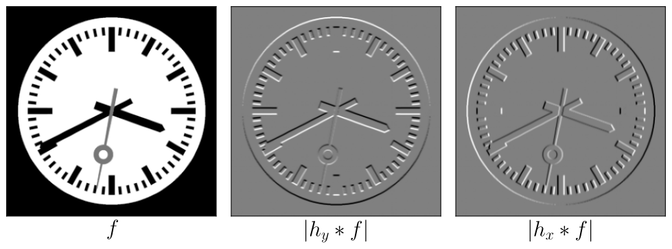
Figure 3:Horizontal and vertical Sobel operator.
Magnitude and angle
From the operators above, we also define:
the magnitude of the edge, which can be interpreted as the “fusion” of the horizontal and vertical Sobel operator:
In Figure 4, all the edges appear with the same color, whatever their orientation.
the angle of the edge:
In Figure 4, the color of the edges corresponds to the edge orientation. Especially, verticals are in red, and horizontals in cyan.
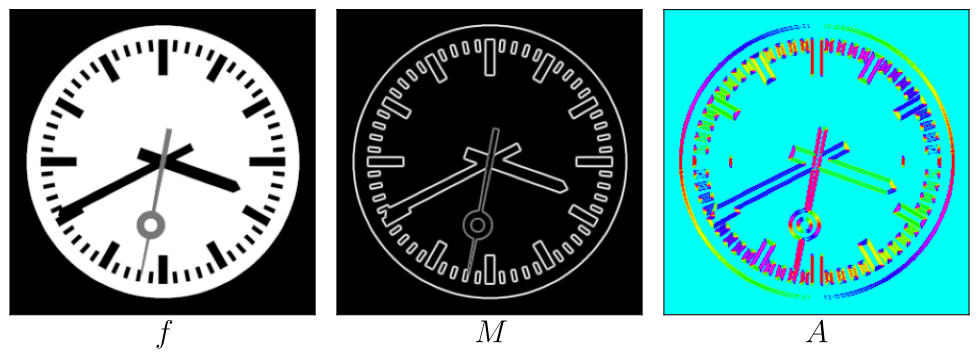
Figure 4:Magnitude and angle of the Sobel operator.
Thresholding
In some cases, it would be useful to detect the most important edges. To do that, one can threshold the magnitude to keep only the large values of the gradients. As you can see in Figure 5, the threshold makes the second hand disappear. Indeed, the magnitude is lower than other parts of the image because the second hand is gray and not black.
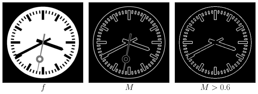
Figure 5:Thresholding the magnitude of the Sobel operator makes the second hands disappear!
The impact of noise
Noise in an image essentially brings great variations in brightness between pixels. Therefore, the gradient operator, which are based on the derivative, are very sensitive to the noise (see Figure 6). Then it may be useful to denoise the image before edge detection.
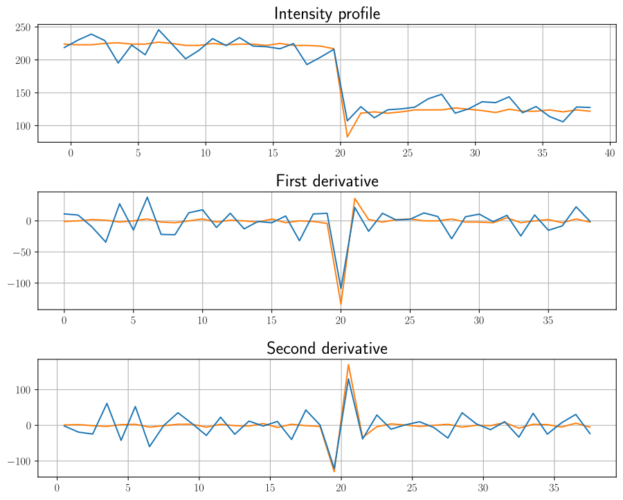
Figure 6:Consequence of noise on the brightness profile and its derivatives (orange: non-noisy profiles, blue: noisy profiles).
In Figure 7, a small blur filter is used before the Sobel filter: the result is much cleaner than without the use of the mean filter.
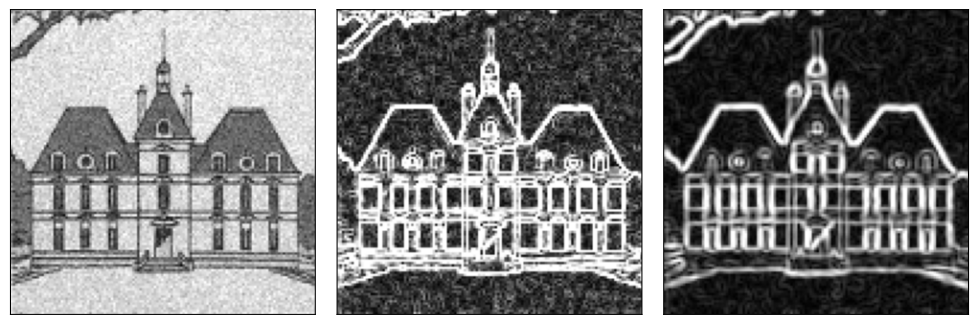
Figure 7:Left: noisy image. Center: Sobel operator (magnitude). Right: Sobel operator applied on the result of a 3×3 mean filter.
Advanced methods
Following the gradient operator, new methods have been proposed to improve edge detection by taking into account the noise and the nature of the edges:
the Marr-Hildreth detector [Marr & Hildreth 1980],
the Canny detector [Canny 1986].
Marr-Hildreth Detector
The Marr-Hildreth detector consists of:
applying a Gaussian filter on the image to reduce noise (this is similar to a mean filter), leading to an image ,
computing the Laplacian (second derivative) on the softened image (this is implemented with a convolution),
determining the zero-crossings of the result.
As , the first two steps are merged into a single convolution by . The filter is the second derivative of a Gaussian:
The filter is represented Figure 8. It is also called “LoG” for Laplacian of Gaussian (no French equivalent) or Mexican hat (for the resemblance to a sombrero).
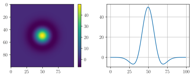
Figure 8:Laplacian of Gaussian (left: as an image, right: profile along an axis).
The zero-crossings in the image resulting from the LoG convolution are given by searching for changes of sign in the intensity of two pixels.
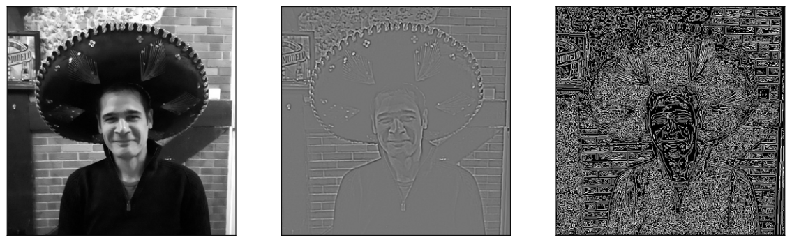
Figure 9 gives an example of applying the Marr-Hlidreth detector.
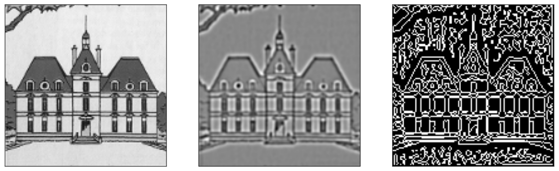
Figure 9:Marr-Hildreth Detector. Left: original image, center: result of the LoG filter, right: detection of the zeros crossings.
Canny Detector
According to Canny, a good detector should serve the following purposes:
all edges should be found,
there should be a minimum of spurious responses,
the edges must be correctly localized (i.e. the distance between a detected point and the true point of the edge must be as small as possible),
the thickness of the detected edges must be 1 pixel (therefore only one point must be detected for each true point of the edge).
Canny expressed these goals in mathematical form and came up with optimal solutions verifying these goals. The Canny detector algorithm follows the four steps detailed below.
The image is first smoothed with a Gaussian filter to reduce noise. This is done by using a convolution with a Gaussian kernel to obtain an image .
The gradient of the image is calculated (amplitude and angle):
Non-maxima are removed from the amplitude. This means that excessively large outlines in are replaced by thinner outlines. For this, we apply the algorithm below:
For each pixel in :
Choose the direction (vertical, horizontal or one of the two diagonals) the closest to
If is lower than one of its neighbors in the chosen direction then cancel the gradient:
The last step consists of thresholding by hysteresis for the bad edges. Two thresholds are therefore defined () and the algorithm below is applied:
For each pixel in :
If then is an edge
If then is an edge if and only if it is neighbor of an edge pixel
If then is not an edge
Figure 11 gives an example of Canny edge detection.
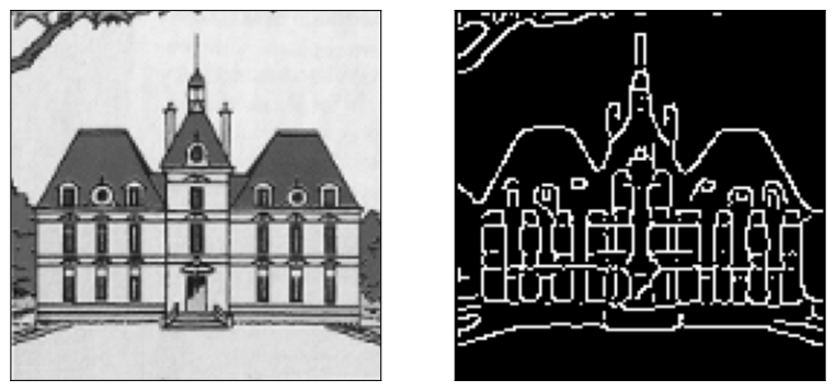
Figure 11:Canny Detector.
Comparison
Figure 12 shows the results of the Sobel, Marr-Hildreth and Canny detectors on an image. A detail is given in Figure 13 and compares Marr-Hildreth and Canny detectors: one can see that the edges detected with Canny detector are better localized.
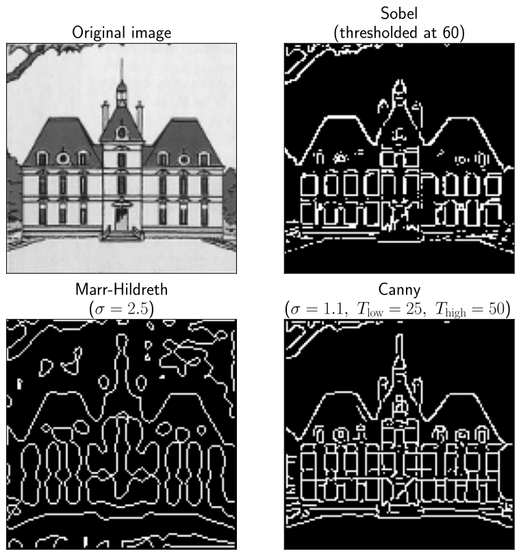
Figure 12:Comparison of Sobel, Marr-Hildreth and Canny detectors.
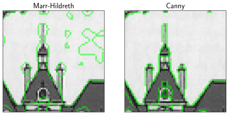
Figure 13:Comparison between Marr-Hildreth and Canny detectors (zoom). The edges are shown in green.