Sampling - Basics of Image Processing

In this section we study the consequence of a digital acquisition of an image, especially the effect due to the sampling.

Mathematical model of sampling¶

We see in Image acquisition that sensors used a matrix of single sensors to acquire the image. Mathematically, the acquired image $g$ can be modeled as:

f = o \times ш_T

Note that this equation is given in the analog domain: the three images $f$ , $o$ and $ш_T$ are not digital (they are continuous functions) and they are of infinite size. The image $o$ is the observed scene and $ш_T$ is a mathematical function defined as

ш_T(m,n) = \sum_{k=-\infty}^{+\infty} \sum_{\ell=-\infty}^{+\infty} \delta(m-kT, n-\ell T).

The equivalent 1D signal of $ш_T$ is called a “Dirac comb”. $T$ is called the sampling period and corresponds to the distance between the pixels in the sensor. In 2D, $ш_T$ corresponds to a field of Dirac pulses with a distance $T$ between two neighboring Dirac pulses.

Applying the Fourier transform on the model yields:

\mathcal{F}[f] = \mathcal{F}[o] * \mathcal{F}[ш_T].

The Fourier transform of $ш_T$ is $\mathcal{F}[ш_T] = ш_F$ where $F=1/T$ is called the sampling frequency.

Because of the convolution, the Fourier transform of the acquired scene is a periodical reproduction of the Fourier transform of the observed scene. Figure 1 illustrates the acquisition model in the spatial and Fourier domains.

Illustration of the effect of sampling on an (analog) observed image.
The images are of infinite support.
The dots are Dirac pulses \delta.
First row: spatial domain;
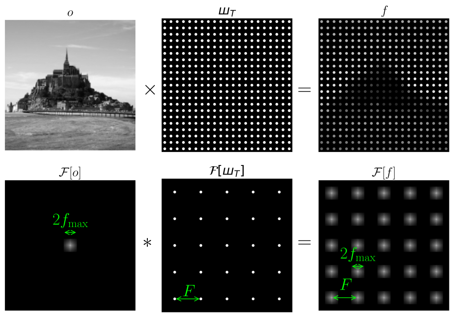
Second row: Fourier domain. — Figure 1:Illustration of the effect of sampling on an (analog) observed image. The images are of infinite support. The dots are Dirac pulses $\delta$ . First row: spatial domain; Second row: Fourier domain.

One can see clearly in Figure 1 the periodical reproduction of the Fourier transform of the image. It is important to see that the reproductions can overlap, depending on two variables:

the “size” of the spectrum, which is actually equal to $2f_\mathrm{max}$ where $f_\mathrm{max}$ is the maximal frequency in the spectrum,
the distance between each reproductions in the Fourier space, which is actually the sampling frequency $F$ .

Aliasing and anti-aliasing¶

The overlap of the spectrum has a major drawback: because high frequencies overlap over middle frequencies, the frequency content of the image change, so the image itself changes.

The consequence of spectrum overlapping is a phenomenon called aliasing (an example is shown in Figure 12 in section Sampling).

To prevent aliasing, it is mandatory to satisfy

F > 2 f_\mathrm{max}.

This condition is at the heart of the samping theorem, edicted by [Shannon, 1948], which can be written as the fact that an analog image with maximal frequency $f_\mathrm{max}$ has to be sampled at frequency $F > 2 f_\mathrm{max}$ to prevent aliasing.

In practice, aliasing is avoided by implementing a low-pass filter before sampling so as to reduce the maximal frequency of the image to $F/2$ . The low-pass filter can be provided by the acquisition device (for example with a lens in front of the sensor that blurs the image) or by implementing the so-called anti-aliasing (low-pass) filter.