Create a simple image

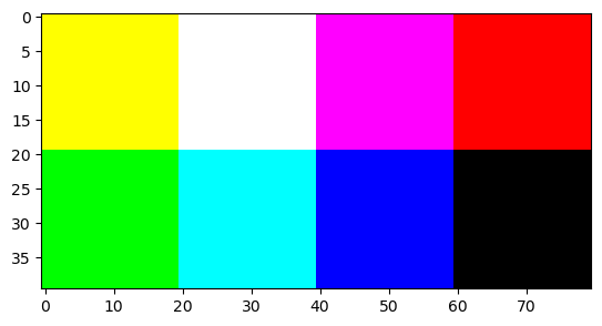
An RGB image is encoded in the form of a three-dimensional array: the first two dimensions are the spatial dimensions of the image, the third corresponds to the bands.

Create the array corresponding to the RGB image $40 \times 80$ sketched Figure 1:
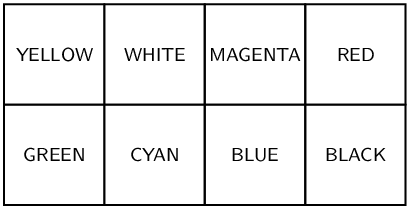
Figure 1:A simple image.
To do this, create first a black image with the correct dimensions (numpy.zeros generates an array filled with zeros). Then assign the desired value to the elements of the matrix, proceeding band by band, by using for example:
```
f[m1:m2, n1:n2, b] = x
```
This statement assigns the value x to the pixels of the band b located between the rows m1 and m2-1 and the columns n1 and n2-1 (in Python, indices starts at 0).

Correction¶

Objectives¶

Synthesize an RGB image (and know, for example, that yellow = green + red).
Manipulate the value / color correspondence.
Use the : operator.

Image synthesis¶

As usual, do not forget the modules:

import numpy as np
import matplotlib.pyplot as plt

The image is composed of blocks of homogeneous color with size 20 × 20 pixels, so as to form an image of 40 × 80 pixels. Also, it contains three bands as it is an RGB image. Therefore we create an array f of size 40 × 80 × 3:

f = np.zeros((40,80,3))

We use Additive color to create the colors. Thus, yellow is obtained by combining green and red.

f[ 0:20 ,   :   , 0 ] = 1   # Red band = band 0   (top row: pixels 0 to 19)
f[  :   ,  0:40 , 1 ] = 1   # Green band = band 1 (the two columns on the left)
f[  :   , 20:60 , 2 ] = 1   # Blue band = band 2  (the two columns at the center)

The bands can be displayed separately:

plt.figure(figsize=(15,7))

plt.subplot(1,3,1)
plt.imshow(f[:,:,0], cmap="gray")
plt.title('Red band')

plt.subplot(1,3,2)
plt.imshow(f[:,:,1], cmap="gray")
plt.title('Green band')

plt.subplot(1,3,3)
plt.imshow(f[:,:,2], cmap="gray")
plt.title('Blue band')

plt.show()

And finally the color image:

plt.imshow(f)
plt.show()