Display a saved image

Open a new notebook.
Download the image 4.2.03.tiff (available online) in the same folder as your notebook.
Write in the notebook the following statements to allow the use of the modules skimage.io and matplotlib.pyplot which are renamed io and plt.
```
import skimage.io as io
import matplotlib.pyplot as plt
```
The names io and plt are conventional names, but you can define other terms.

Load :

f = io.imread("4.2.03.tiff")

and display it:

plt.imshow(f)

What are the dimensions (in pixels) of the image?

The conversion of a color image with pixel values $r$ , $g$ , $b$ to a grayscale image with pixel intensity $x$ is made through the transformation

x = 0.2125 \, r + 0.7154 \, g + 0.0721 \, b.

The coefficients have been obtained by psychovisual studies and guarantee that $x\in[0,1]$ if $r,g,b\in[0,1]$ .

Convert the color image to grayscale (skimage.color.rgb2gray) then display it. Note that rgb2gray is a function in the module skimage.color. To use the function, import the module before using the function, as for example:
```
import skimage.color as color
clr.rgb2gray(...)
```
Print the intensity of the top-left pixel (which is at position $(0,0)$ ) by typing g[0,0].
Print the intensities of the five first pixels of the second row by typing g[1,0:5], which extract from g the pixels at row 1 and columns 0 to 4 (the last index is not reached).
Print the intensities of all the pixels in the third row by typing g[2,:], which extract from g the pixels at row 2 and all the columns.

The natural representation of an image is a two-dimensional display where the intensity of the pixels is given by a color. However, an image can also be seen as a three-dimensional curve, opening the way to new interpretations.

Extract a row or a column of pixels from the image, then display this brightness profile as a signal (matplotlib.pyplot.plot). Do you manage to find in this profile the different areas of the image?

Correction¶

Objectives¶

Use functions and modules.
Know how to load and display an image, and use a colormap.
Display the size of an image.
Convert an image to grayscale.
Use the : operator.
understand that an image is also a 2D signal.

Modules¶

The use of the function ccc available in the submodule bbb of the module aaa writes aaa.bbb.ccc. I am sure you agree this is a bit long to write, that is why we usually rename the submodule to something shorter. Thus, the following instructions rename skimage.io to io, and matplotlib.pyplot to plt:

import skimage.io as io
import matplotlib.pyplot as plt

The three modules used in this course are:

Numpy (scientific programming),
Scikit-image (image processing),
Matplotlib (display).

Refer to the documentation on these websites to get the syntax of the functions.

Display the color image¶

Now you can load the image 4.2.03.tiff. I load it directly from the website, but you can download it on your computer..

f = io.imread("http://sipi.usc.edu/database/download.php?vol=misc&img=4.2.03")

and display it (I take this opportunity to add a title):

plt.imshow(f)
plt.title('4.2.03.tiff (Mandrill)')
plt.show()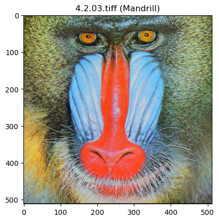

The function plt.show() is the correct way to show the image.

The image dimensions can be read on the displayed image: a little more than 500 pixels per side, and 3 bands since the image is in color. A more precise alternative is to use the shape function:

print(f.shape)

(512, 512, 3)

So the image if of size 512 × 512, with 3 bands.

Conversion to grayscale¶

We need to import a new module (I am doing this at this point, but it is recommended to import all modules at the beginning of the notebook).

import skimage.color as color

g = color.rgb2gray(f)
plt.imshow(g)
plt.title('Mandrill (grayscale)')
plt.show()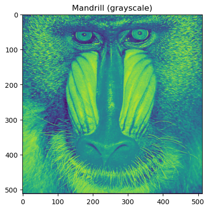

What’s that weird grayscale image? It’s rather green... 😲

This actually is a grayscale image (the image has only one band). But the default colormap provided with imshow is a gradient of blue and green. To display it in real gray levels, you must specify the option cmap in imshow. A large number of palettes are available (see catalog); here we choose the classic gray:

plt.imshow(g, cmap="gray")
plt.title('Mandrill (grayscale)')
plt.show()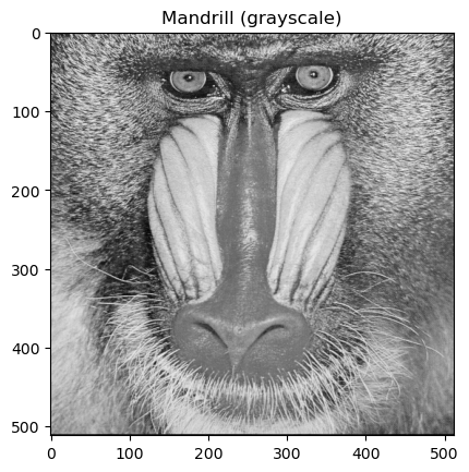

Phew! 😅

The grayscale image has intensities in this range:

print(f"Min : {g.min()}")
print(f"Max : {g.max()}")

Min : 0.0
Max : 0.9116803921568628

The range of colors can also be redefined by specifying the intensities corresponding to black (vmin) and white (vmax):

plt.imshow(g, vmin=0.0, vmax=0.5, cmap="gray");
plt.title("Intensity range = [0.0, 0.5]");
plt.show()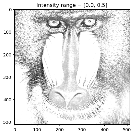

Extraction of pixels¶

The syntax g[a:b,c:d] extract pixels located between rows a and b--1 and columns c and d--1. If a or c is not given, then it is considered to be 0. If b or d is not given, then it is considered to be the maximal index in the dimension.

Then we have the instensity of top-left pixel:

g[0,0]

np.float64(0.5775650980392157)

The intensities of the five first pixels of the second row:

g[1,0:5]

array([0.46821647, 0.39396314, 0.15052863, 0.27128118, 0.3509451 ])

And the intensities of all the pixels in the third row:

g[2,:]

array([0.29887137, 0.45405412, 0.17520392, 0.18225216, 0.39513529,
       0.23370078, 0.23346275, 0.18306275, 0.44279098, 0.42749882,
       0.19147922, 0.23552588, 0.28236667, 0.14554353, 0.10365373,
       0.20003569, 0.47681922, 0.41969843, 0.38021059, 0.22593216,
       0.28821765, 0.20411412, 0.16150392, 0.25885922, 0.3675949 ,
       0.70087843, 0.80062784, 0.69879137, 0.3542451 , 0.18072471,
       0.37092039, 0.66425961, 0.62859882, 0.32563176, 0.48865843,
       0.44584078, 0.43163216, 0.41797137, 0.4346651 , 0.50814902,
       0.29834   , 0.53164941, 0.52597647, 0.48358314, 0.55389647,
       0.58781529, 0.5523349 , 0.56919608, 0.32072275, 0.47438745,
       0.57285569, 0.25036235, 0.34582863, 0.3136149 , 0.38447255,
       0.37164275, 0.33711451, 0.67537804, 0.59824706, 0.62892549,
       0.54611451, 0.59752706, 0.40229412, 0.2953298 , 0.64953529,
       0.65788039, 0.24202118, 0.36884667, 0.49252118, 0.79315843,
       0.70304157, 0.46462706, 0.42678275, 0.25671647, 0.19072196,
       0.64614784, 0.66011961, 0.35292157, 0.57037412, 0.50863059,
       0.29234667, 0.49992588, 0.7499898 , 0.60244275, 0.55461333,
       0.58998824, 0.47794706, 0.31540235, 0.47809922, 0.24272667,
       0.52286   , 0.78632667, 0.70392667, 0.3449149 , 0.32193765,
       0.40283765, 0.33996588, 0.25855725, 0.46996627, 0.56721255,
       0.66268706, 0.26738078, 0.62769373, 0.57931686, 0.34050745,
       0.32190706, 0.17445294, 0.29652902, 0.46807725, 0.59419804,
       0.65354157, 0.55356863, 0.45248588, 0.63711373, 0.78667608,
       0.78139176, 0.66867098, 0.62541686, 0.64168824, 0.50473098,
       0.21474   , 0.46951373, 0.80832078, 0.55386   , 0.74174588,
       0.74282902, 0.42696157, 0.55508784, 0.79211451, 0.65287216,
       0.30708235, 0.61376431, 0.77478275, 0.34201961, 0.26216392,
       0.26048941, 0.34937765, 0.32378039, 0.60389686, 0.48542196,
       0.47154392, 0.53828667, 0.57594   , 0.60560745, 0.56346784,
       0.4943749 , 0.55253725, 0.49998745, 0.73936353, 0.46750078,
       0.35117451, 0.64160078, 0.50857294, 0.67457882, 0.28412471,
       0.31143451, 0.26363176, 0.40436863, 0.20817922, 0.45073765,
       0.24656078, 0.20288588, 0.44887765, 0.52612471, 0.57509843,
       0.70517725, 0.31155529, 0.44951725, 0.32749373, 0.45062392,
       0.22434784, 0.21253137, 0.53796627, 0.58654235, 0.51004549,
       0.35401255, 0.34762314, 0.52055216, 0.3524502 , 0.20716549,
       0.55764588, 0.55081412, 0.53530706, 0.73204196, 0.72333333,
       0.43177686, 0.5625302 , 0.57672157, 0.68679882, 0.49665098,
       0.32977137, 0.61064471, 0.57949647, 0.71874471, 0.60622392,
       0.45755961, 0.47033333, 0.6539451 , 0.71454745, 0.61620275,
       0.59436353, 0.4811651 , 0.40566353, 0.29167176, 0.49708235,
       0.52531412, 0.33124627, 0.56904824, 0.54893294, 0.44701686,
       0.42592863, 0.39929843, 0.46948353, 0.26834902, 0.37489725,
       0.65960863, 0.32994863, 0.29597843, 0.48790157, 0.51648039,
       0.30926745, 0.40897059, 0.70658431, 0.68584392, 0.31943608,
       0.51457098, 0.68033098, 0.44309608, 0.21460941, 0.5708051 ,
       0.30841569, 0.12148471, 0.18900745, 0.23111176, 0.35617373,
       0.63064078, 0.62157843, 0.4543251 , 0.5868102 , 0.63134549,
       0.35060667, 0.51869843, 0.23740824, 0.44154902, 0.60687922,
       0.63498353, 0.25839373, 0.49051725, 0.60004118, 0.68548235,
       0.55514078, 0.73690902, 0.7019949 , 0.49392235, 0.38955451,
       0.27914118, 0.4273651 , 0.41536784, 0.25250863, 0.49767843,
       0.34849373, 0.29043529, 0.27982392, 0.55084627, 0.62948549,
       0.55583882, 0.27288784, 0.56052235, 0.66894   , 0.38284314,
       0.43967529, 0.2774502 , 0.26997804, 0.28804706, 0.45563294,
       0.50055765, 0.74024863, 0.61882902, 0.41892431, 0.56081059,
       0.60970863, 0.71147412, 0.75721647, 0.61909059, 0.65936275,
       0.59161608, 0.44407569, 0.39787529, 0.42114314, 0.48729686,
       0.37464902, 0.30955882, 0.33337961, 0.64318431, 0.51892157,
       0.58090078, 0.55057686, 0.4523302 , 0.52688392, 0.31417373,
       0.27305843, 0.43903255, 0.60187137, 0.61762431, 0.42226471,
       0.31401608, 0.39641686, 0.61858353, 0.53392157, 0.30225922,
       0.46834196, 0.40980824, 0.37164039, 0.4239549 , 0.37574392,
       0.51241843, 0.51272314, 0.58368431, 0.59460706, 0.33814078,
       0.63098902, 0.65416745, 0.50459647, 0.64279059, 0.6570851 ,
       0.49102588, 0.65684078, 0.50505098, 0.23141804, 0.20387608,
       0.49046824, 0.27620549, 0.43045922, 0.55709804, 0.74841216,
       0.64306627, 0.70716745, 0.73133412, 0.36815294, 0.65667098,
       0.5889549 , 0.61651529, 0.46833451, 0.22244235, 0.28930235,
       0.42694039, 0.39629882, 0.64588667, 0.3499502 , 0.28574039,
       0.42263804, 0.29248078, 0.2453702 , 0.36597843, 0.49566784,
       0.46113333, 0.30190118, 0.42555647, 0.69971176, 0.70840078,
       0.48582118, 0.2531898 , 0.18831843, 0.40755412, 0.44412275,
       0.32613882, 0.53831333, 0.42903098, 0.6589251 , 0.72162392,
       0.5700298 , 0.67195373, 0.71072235, 0.58323725, 0.38245529,
       0.66597765, 0.62270745, 0.4811502 , 0.64357294, 0.6911302 ,
       0.46150588, 0.17370039, 0.15491882, 0.28686196, 0.61202824,
       0.73338157, 0.74530902, 0.65347608, 0.65087098, 0.42826314,
       0.71725647, 0.7201349 , 0.49603922, 0.37203765, 0.47086471,
       0.62737216, 0.58209098, 0.68531843, 0.58510431, 0.47664118,
       0.61493765, 0.59421137, 0.3861098 , 0.38211294, 0.7358498 ,
       0.41067137, 0.47752078, 0.74665765, 0.70586902, 0.31205961,
       0.30702824, 0.3080549 , 0.51851961, 0.47489216, 0.53479569,
       0.53559843, 0.65944471, 0.53486235, 0.52856706, 0.48515569,
       0.26078157, 0.65548824, 0.5378302 , 0.31735647, 0.4392051 ,
       0.40995098, 0.48542941, 0.62159569, 0.52709922, 0.35710235,
       0.6793502 , 0.78834275, 0.77483686, 0.79081216, 0.61601529,
       0.51214941, 0.51948667, 0.42916549, 0.48015098, 0.44226784,
       0.54357725, 0.59253137, 0.60061098, 0.42591373, 0.65666078,
       0.76882392, 0.78575882, 0.60957451, 0.4676651 , 0.60167059,
       0.80047137, 0.72537804, 0.43510392, 0.62954549, 0.60625098,
       0.42893529, 0.76703882, 0.82513882, 0.65869098, 0.46839176,
       0.48753216, 0.5579451 , 0.60944706, 0.75215451, 0.71587137,
       0.70802667, 0.54521608, 0.35049961, 0.61257843, 0.74617333,
       0.81649373, 0.74969255, 0.62443255, 0.32151059, 0.65618471,
       0.66241922, 0.31468392, 0.44372863, 0.63504941, 0.68894196,
       0.72772   , 0.77370588, 0.60649843, 0.32699569, 0.50390627,
       0.40383373, 0.24985725, 0.38521412, 0.49977216, 0.68890275,
       0.69251961, 0.73503176, 0.59991294, 0.69705137, 0.40038588,
       0.37019922, 0.17809255, 0.19862824, 0.33471961, 0.27111333,
       0.26034118, 0.5153349 , 0.59366039, 0.37718471, 0.30610902,
       0.40581451, 0.54923098, 0.49104588, 0.39092235, 0.38469098,
       0.34957098, 0.31829373])

Brightness profile¶

I choose a horizontal cut on the 200^th line of the image:

cut = 200          # Cut location
profil = g[cut,:]  # Extract all the pixels of the row 'cut' in the image g

Now we can display the brightness profile...

plt.figure(figsize=(10,5))           # New figure with specific display size

plt.subplot(1,2,1)                   # Plot on the left
plt.plot(profil,'b')                 # Brightness profile
plt.title("Brightness profile")      # Title

plt.subplot(1,2,2)                   # Image on the right
plt.imshow(g, cmap="gray")           # Image
plt.plot((0,511), (cut,cut), 'b')    # Cut line in blue
plt.title("Mandrill")                # Title

plt.show()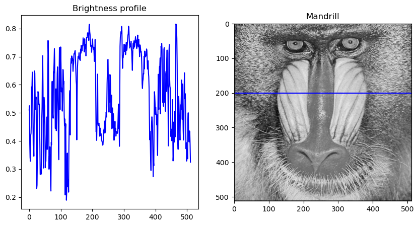

Do you see on the profile the Mandrill’s nose and the protruding ridges on its sides?