(binary=applications)=
Applications
The four morphological tools seen above are the elementary operations for more complex processing. In this section, we focus on some specific processings, others are given by [Bloch 2005, chapter 6].
Top-hat transform
The top-hat transformation (French: transformée du chapeau haut-de-forme) keeps in the image only the objects that are narrower than the structuring element. There are two dual top-hat transforms:
The white top-hat transform is defined as the difference between the image and its opening by the structuring element :
The black top-hat transform is defined as the difference between the closing by the structuring element and the image:
Figure 1 shows the effect of a white top-hat transform (only the white objects narrower than the structuring element are kept) and a black top-hat transform (only the black objects narrower than the structuring element are kept). Note that the structuring element, present in the original image, is not kept because it is not narrower than itself. The results also show many of very small artifacts that can be easily removed by discarding the objects whose size is smaller than a predefined threshold.
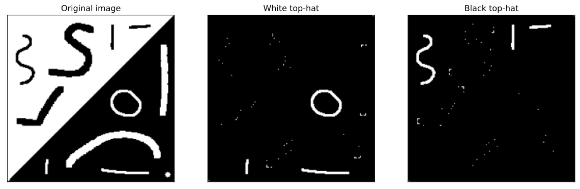
Figure 1:Example of a white and black top-hat transforms with a disk of radius 3 pixels as structuring element (the latter is visible in the bottom-right corner of the original image).
Granulometry
Granulometry (French: granulométrie) is an approach that successively selects particles of increasing sizes in a binary image. It consists of successive openings of an image by a sequence of structural elements of increasing size (usually, ) where is a disk).
At each stage of opening, the finer details are successively eliminated, and the area of the image is reduced (the area is the total number of pixels in the objects.).
Figure 3 shows the granulometry function obtained on the binary image of Figure 2 by openings with a disk of different sizes. When the size of the opening corresponds to the characteristic size of most objects, a jump appears in the curve.
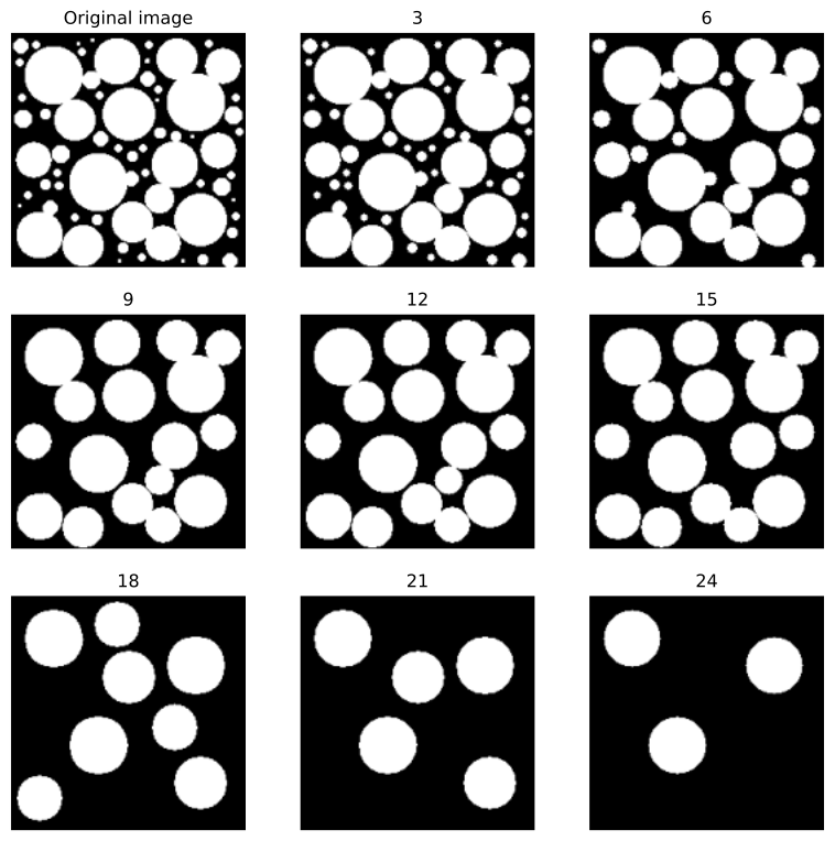
Figure 2:The original image and the corresponding openings by the successive structuring element (a disk).
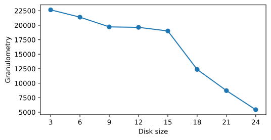
Figure 3:The granulometry function.
Hit-or-miss transform
The hit-or-miss transform (French: transformée tout-ou-rien) is used to detect objects of a particular shape. Contrary to the transformations seen so far, the hit-or-miss transform examines configurations where certain pixels verify a relationship with the object and others verify a relationship with the complement of the object. Thus the structuring element of this transformation is composed of two elements and (disjoint but with the same origin).
The result of the hit-or-miss transform is the intersection of the two sets given by:
the erosion of the image by : ,
the erosion of the image background by :
The hit-or-miss transform by the two structuring elements and is noted :
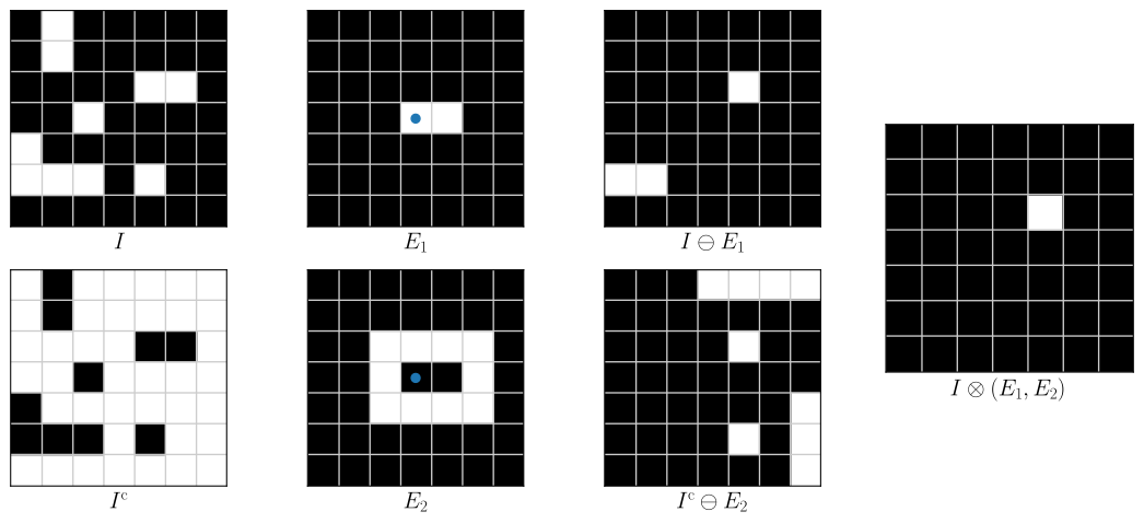
Figure 4:Example of a hit-or-miss transform applied on the image by the structuring elements and . The origin of the structuring elements are marked by the blue dot. Some white pixels in comes from the background outside which is considered as white.
Skeleton
The skeleton (French: squelette) is a useful notion in pattern recognition: it is a “compact” form of the objects (thin lines centered within the objects), with the same number of connected components and the same number of holes.
From a structuring element , let us define :
The skeleton of image is defined as:
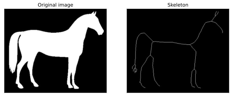
Figure 5:Skeleton of the image .