Denoising - Basics of Image Processing

Denoising (French: débruitage) consists in reducing noise in an image. Note that it is often not possible to completely cancel the noise. We start this section by listing the most common noise models, then we present some denoising methods.

Noise sources¶

The main sources of noise in digital images are during the acquisition (quantity of photons collected too low, sensor temperature...) or during any transmission (echoes and atmospheric distortions in wireless communication). In some cases, noise is also considered to model the inaccuracies in the mathematical model of image formation, the latter being necessarily different compared to reality, like any physical model!

The noise is by nature a random phenomenon, it is modelled by a probability density which represents the intensity distribution of the noise.

In the following, we denote by $y$ the observed (and noisy) image, $b$ the noise and $x$ the non-noisy image.

Additive Gaussian white noise¶

Additive white Gaussian noise (AWGN, in French: bruit blanc gaussien additif) models each pixel $(m,n)$ of the observation $y$ by the sum of the pixel $(m,n)$ of the noiseless image $x$ and of a pixel of the noise $b$ :

\forall\, m,n \quad y(m,n) = x(m,n) + b(m,n)

where $b(m,n) \sim \mathcal{N}(0,\sigma^2)$ .

This model is simple and facilitates calculations. It is used in most applications, including photography.

Poisson Noise¶

Poisson noise (also called shot noise, in French: bruit de Poisson) models the acquisition of photons on a photosite. The number of photons is random and depends on the illumination. The corresponding Poisson process has a mean equals to the illumination. The intensity of each pixel $(m,n)$ of the observation $y$ is:

\forall\, m,n \qquad y(m,n) \sim \mathcal{P}\big(x(m,n)\big).

This model is used in the case of acquisitions with a low number of photons, for example in astronomy.

Salt-and-pepper noise¶

Salt-and-pepper noise (French: bruit poivre et sel), also called less poetically impulse noise, models saturated or dead pixels (due to photosite malfunction or saturation).

\forall\, m,n \quad y(m,n) = \begin{cases} x_\mathrm{min} &\text{with probability}\,p_\mathrm{min}, \\ x_\mathrm{max} &\text{with probability}\,p_\mathrm{max}, \\ x(m,n) &\text{with probability}\,1\!-\!p_\mathrm{min}\!-\!p_\mathrm{max}. \end{cases}

where $x_\mathrm{min}$ and $x_\mathrm{max}$ are the intensity minimum and maximum.

Noise power¶

Figure 2 illustrates the effect of the previous noises on the same image. One can observe that:

for Gaussian noise, the whole image is affected in the same way by the noise,
for Poisson noise, the lighter parts are noisier than the dark parts,
for impulse noise, only a few pixels are modified and they are replaced by black or white pixels.

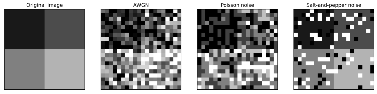
Figure 2:Example of different types of noise (with almost the same power).

Signal-to-noise ratio (SNR, in French: RSB for rapport signal-sur-bruit) is a measure of the noise level. It is defined as the ratio between the power of the non-noisy image over the power of the noise, where the power of an image $x$ is defined by:

P_x = \frac{1}{M \times N} \sum_{m,n} x(m,n)^2

Because SNR is most often expressed on a logarithmic scale (unit: decibel), it is also defined as:

\text{SNR} = 10 \log_{10} \left( \frac{\sum_{m,n} x(m,n)^2}{\sum_{m,n} b(m,n)^2} \right)

For additive noise, another measure exists: the peak signal-to-noise ratio (PSNR) is the ratio of the squared dynamics of the non-noisy image (difference between maximum intensity and minimum intensity) to the power of the noise:

\text{PSNR} = 10 \log_{10} \left( \frac{\Delta x^{\;2}}{\frac{1}{M \times N} \sum_{m,n} b(m,n)^2} \right)

Figure 3 represents the same image corrupted with additive white Gaussian noise, at different SNR and PSNR. As you can see, when the RSB or the PSNR increases, the noise decreases!

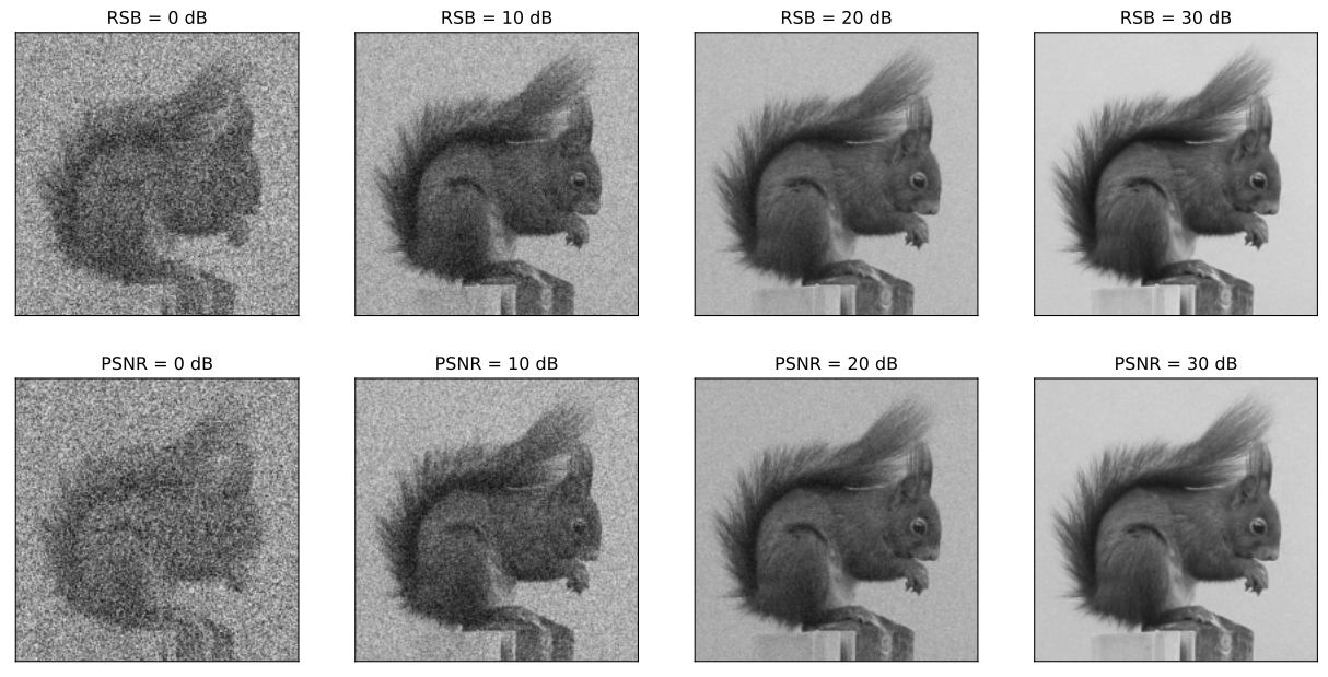
Figure 3:Noisy image at different RSB and PSNR.

Mean filter¶

The mean filter (French: filtre moyenneur) is a very simple denoising method. Each pixel $(m,n)$ of the denoised image $\widehat{x}$ is the average of the pixels of the noisy image $y$ around $(m,n)$ :

\forall m,\,n \quad \widehat{x}(m,n) = \frac{1}{|V_{m,n}|} \sum_{(u,v)\in V_{m,n}} y(u,v)

where

$V_{m,n}$ is the neighbourhood, that is the set of pixels around $(m,n)$ ;
$|V_{m,n}|$ is the cardinality of $V_{m,n}$ , that is, the number of pixels in the neighbourhood.

Figure 4 illustrates the effect of the mean filter for different sizes of the neighbourhood. If the neighbourhood grows, then the noise decreases but at the same time the image becomes more blurry.

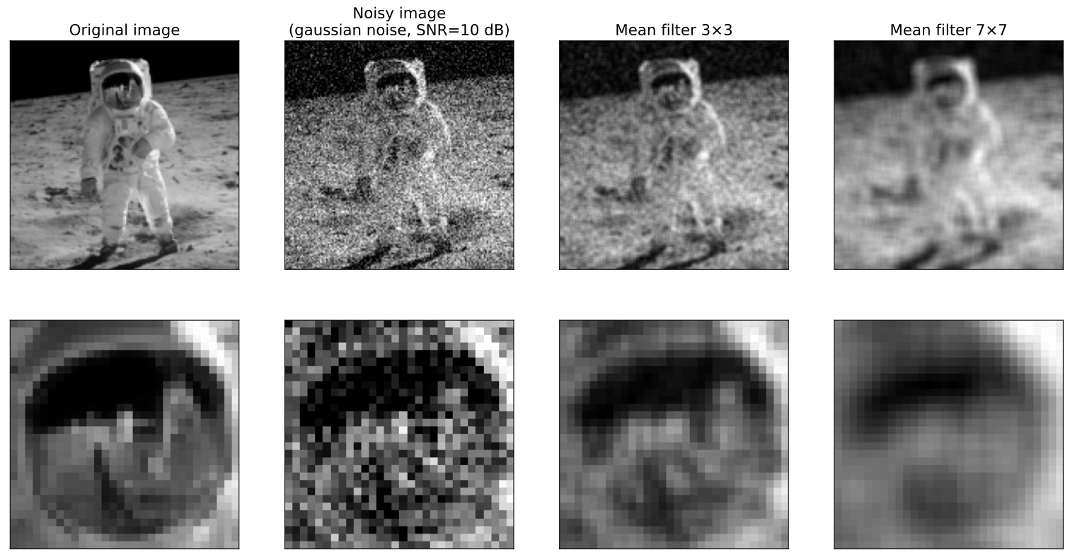
Figure 4:Effect of the size of the mean filter.

The mean filter can be expressed with a convolution product. Indeed, consider the case where the neighbourhood is a square of size $N\times N$ pixels, then the definition of the mean filter gives:

\widehat{x}(m,n) = \frac{1}{N^2} \sum_{(u,v)\in V_{m,n}} y(u,v) = \sum_{u,v} g(m-u,n-v) y(u,v)

where

g(u,v) = \begin{cases} 1/N^2 &\text{if}\, u\in\left\{-\frac{N}{2},\dots,\frac{N}{2}\right\} \,\text{and}\, v\in\left\{-\frac{N}{2},\dots,\frac{N}{2}\right\} \\ 0 &\text{otherwise} \end{cases}

This definition can be extended to any type of kernel $g$ ! For example, Figure 5 gives the result for two different kernels.

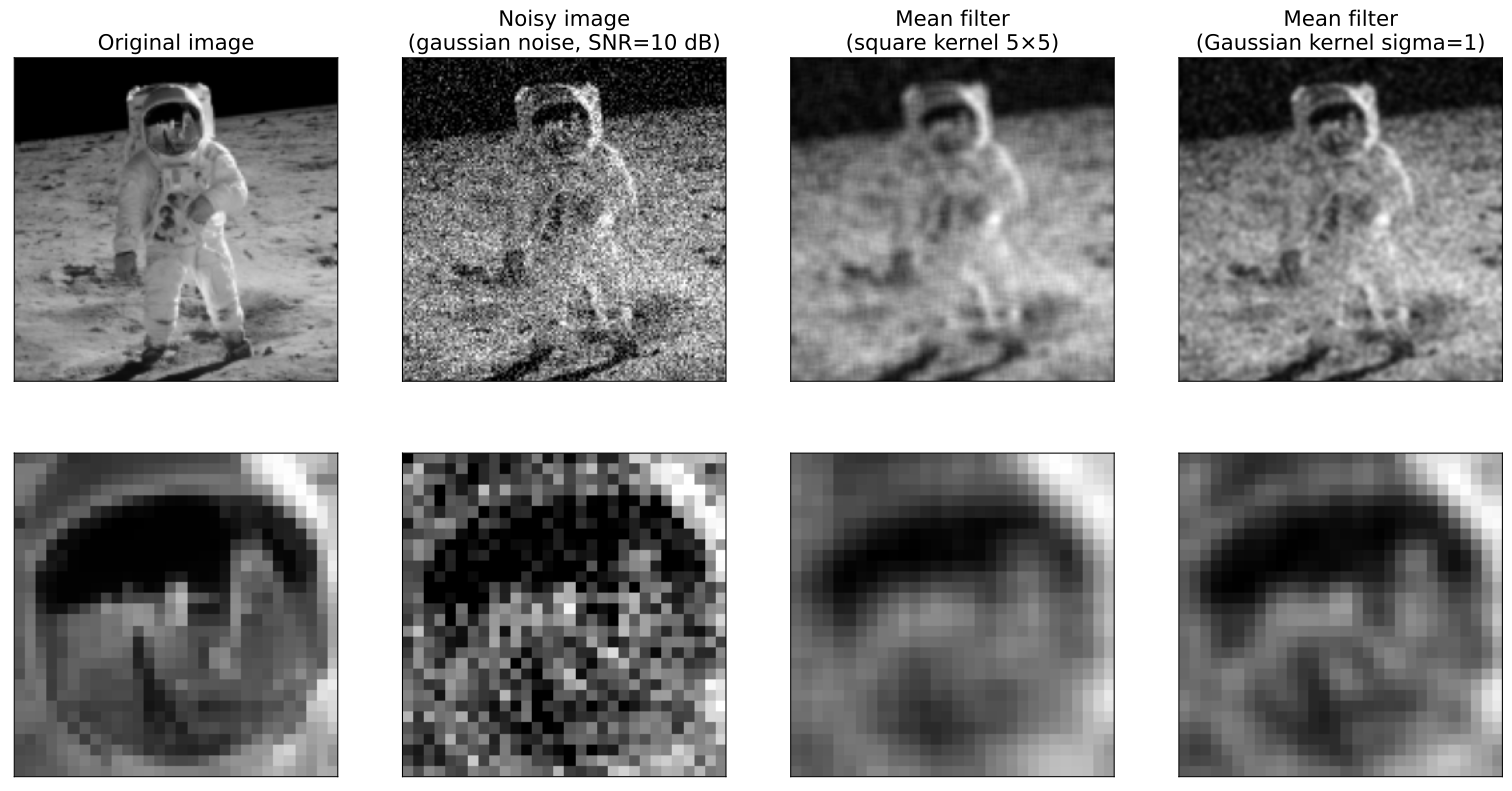
Figure 5:Two mean filters with different kernels.

In summary:

the mean filter calculates the average of the pixels in a neighbourhood,
the mean filter can be written as a convolution,
the noise is reduced by averaging the intensities but the image is blurred.

Median filter¶

The median of a set of numbers is the element $m$ of the set such that there are as many numbers smaller than $m$ as there are numbers larger than $m$ . For example, the median of $\{1,\,2,\,4,\,8,\,16\}$ is 4.

The median filter (French: filtre médian) is defined by:

\forall m,\,n \quad \widehat{x}(m,n) = \mathrm{median}\big(\{y(u,v) \mid (u,v)\in V_{m,n}\}\big)

The median filter is excellent for denoising an image in the case of salt-and-pepper noise because it does not blur the image, as a mean filter would do.

Despite its name, the median filter is not a filter because it does not respect the linearity property. Therefore it cannot be written as a convolution.

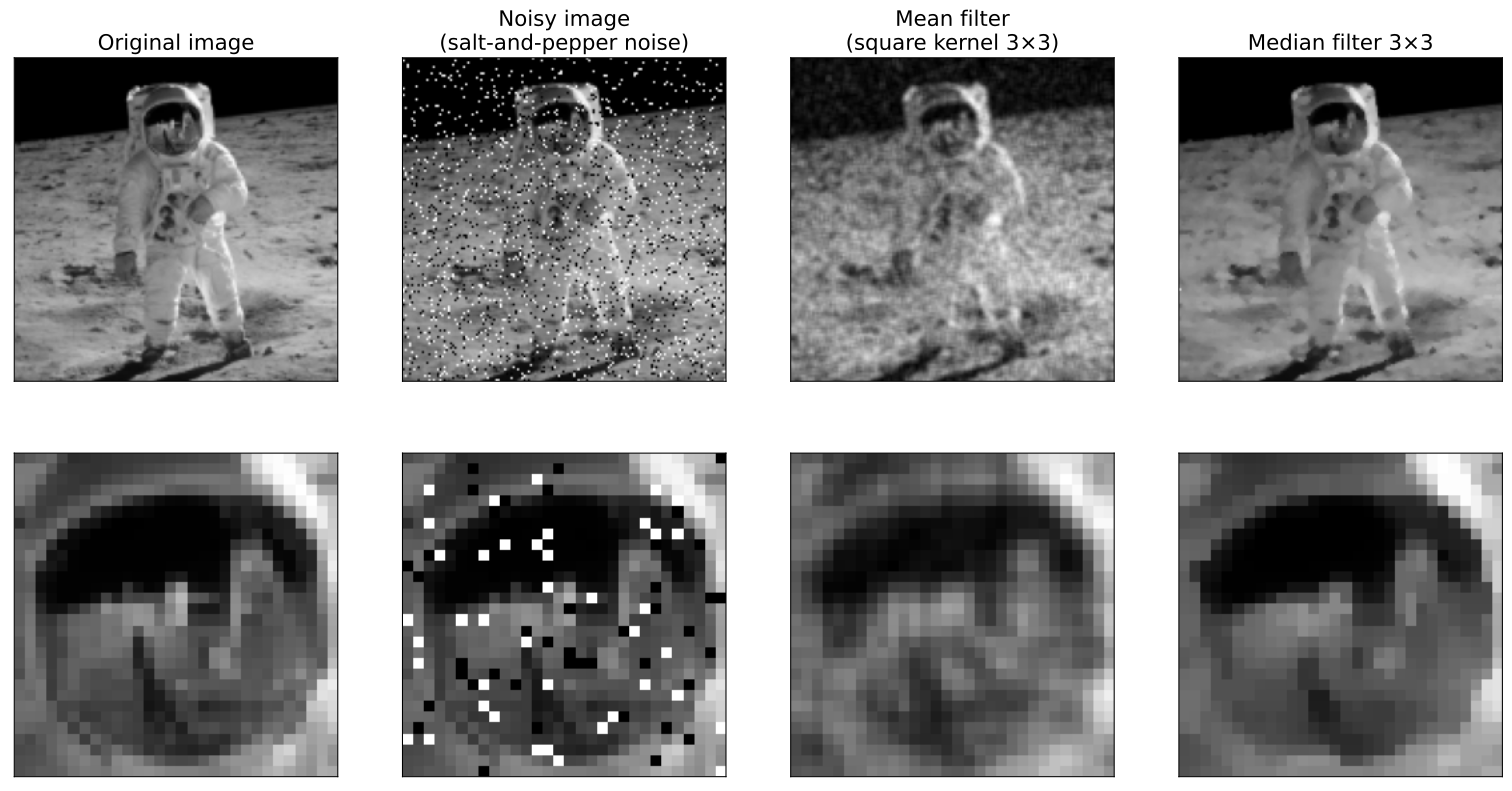
Figure 6:Comparison between a mean filter and a median filter, on an image with salt-and-pepper noise.

Periodic noise filtering¶

Periodic noises are characterized by structures in the Fourier transform. These structures can be removed in the Fourier domain by cancelling the coefficients using a mask. The denoised image is then obtained by an inverse Fourier transform.

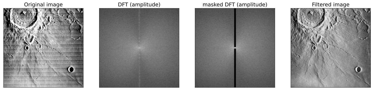
Filtering a periodic noise on a photograph of the Moon:
the image is cleaned of periodic image artefacts. — Figure 7:Filtering a periodic noise on a photograph of the Moon: the image is cleaned of periodic image artefacts.

TV regularization¶

From a certain point of view, the goal of denoising is to obtain an image $\widehat{x}$ not only with small variations in intensity between pixels but also close to the observation $y$ . TV regularization (total variation, French: variation totale) [Rudin et al. 1992, Chambolle 2004] is a denoising method that describes these two objectives by mathematical functions (the so-called “criteria”).

The wish to have a denoised image $\widehat{x}$ close to the observation $y$ results in a “data-fit” criterion (French: critère d’adéquation aux données) which measures the difference between $x$ and $y$ . A classic choice to measure this difference is the least-squares criterion:
$E(x,y) = \sum_{m,n} \left(y(m,n)-x(m,n)\right)^2$
Indeed, for $E$ to decrease, we must find an image $x$ close to $y$ .
The desire to have an image with small variations in intensity results in a “regularization” criterion (French: critère de régularisation) which measures the difference between the neighbouring pixels of $x$ . A simple choice is the “total variation”:
$R(x) = \sum_{m,n} \left|x(m+1,n)-x(m,n)\right| + \sum_{m,n} \left|x(m,n+1)-x(m,n)\right|$
So, for $R$ to decrease, the difference between two consecutive pixels, whether they are in a row or column, must be small. This implies the image $x$ to be nearly constant in intensity.

The goal is then to find the image $x$ which minimizes both the data-fit and the regularization. Mathematically, one look for the image $x$ which minimizes $E(x,y) + \lambda R(x)$ , where $\lambda$ is the “regularization parameter” (French: paramètre de régularisation) which is used to adjust the compromise between the two criteria. The value of $\lambda$ is chosen by the user. Mathematically, we write:

\widehat{x} = \arg\min_x E(x,y) + \lambda R(x)

This comes to an optimization problem, and there are a large number of algorithms to minimize $E(x,y) + \lambda R(x)$ . The choice and description of these algorithms are beyond the scope of the course.

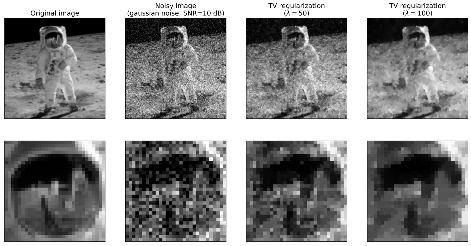
Denoising with TV regularization, for two values of \lambda. — Figure 8:Denoising with TV regularization, for two values of $\lambda$ .