Usually, images acquired by a vision system suffer from degradation that can be modelled as a convolution. For example, some images present a camera shake effect (Figure 1) or a blur due to poor focus (Figure 2). The goal of deconvolution is to cancel the effect of a convolution.
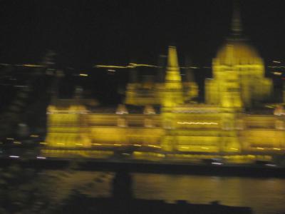
Figure 1:An example of motion blur (the parliament of Budapest shot by a camera).

Figure 2:Hubble’s view of Ganymede in 1996.
The degradation phenomenon is modelled as in Figure 3: The observed image is degraded by the convolution with a PSF and, possibly, by a noise (considered to be additive).
The deconvolution computes a deconvolved image from the observation . We will consider only linear methods, thus deconvolution comes to filtering by :
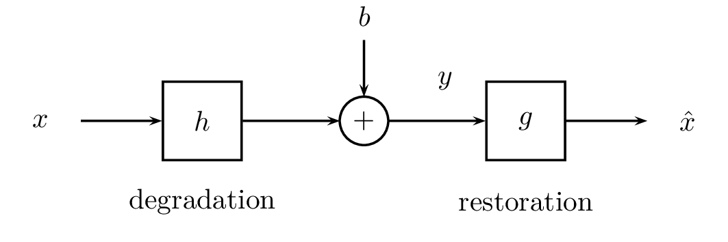
Figure 3:Deconvolution model.
Deconvolution needs a degradation model, thus having knowledge about both and .
The PSF can be estimated by observation, i.e. by finding in the image some factors to estimate . For example, a single point object in the image is . The PSF can also be estimated by experimentation by reproducing the observation conditions in a laboratory. So, the image of a pulse gives an estimate of . Finally, it is also possible to estimate the PSF from a mathematical model of the physics of the observation. Note also that some deconvolution methods estimate the PSF at the same time as : these are called blind deconvolution methods (French: déconvolution myope).
Models for the noise have already been presented in chapter C:denoising.
Inverse filter
The inverse filter is the simplest deconvolution method. Since the degradation is modelled , then this equation becomes in the Fourier domain:
so we can write:
We obtain by calculating the inverse Fourier transform of the previous expression:
As the noise (and therefore its spectrum ) is unknown, we can approximate the expression of by cancelling in the previous expression, and thus get the deconvolved image:
The result of the inverse filter applied on an image is given Figure 4. The result is not usable, and yet the observed image is very little blurred with very little noise!
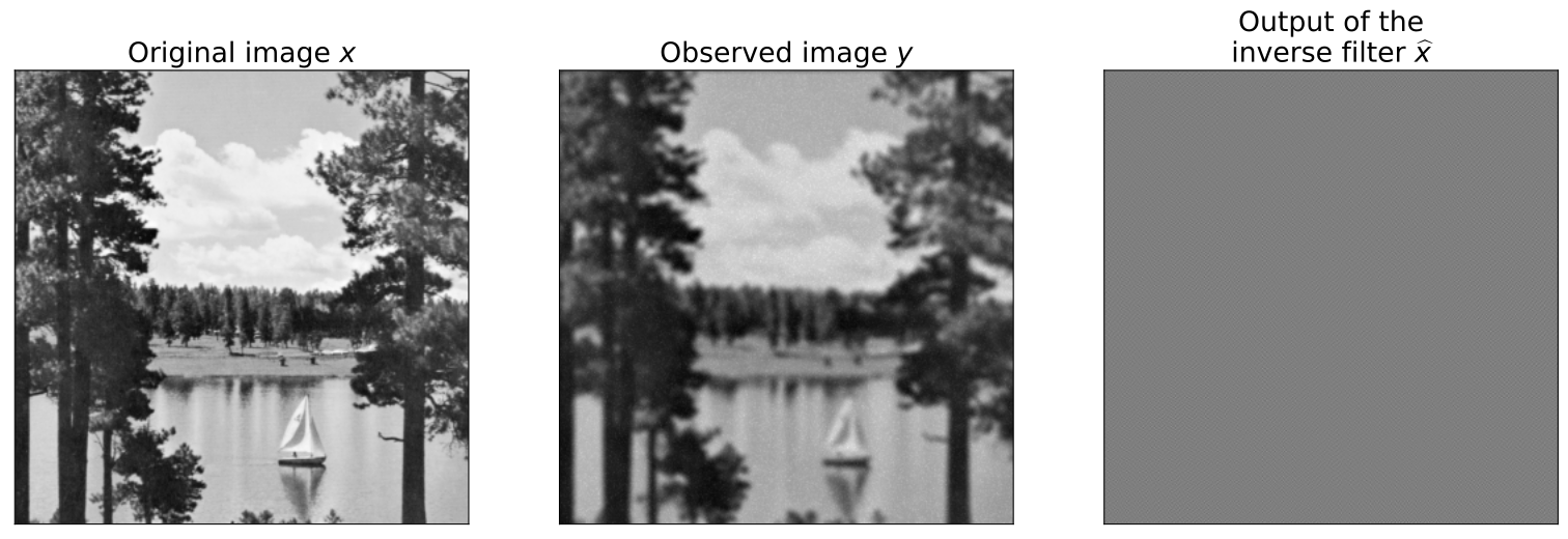
Figure 4:Result of the inverse filter.
The catastrophic result of the inverse filter is due to the fact of having considered the noise to be zero. Indeed, according to the definition of and considering , then:
Thus, the deconvolved image corresponds to with an additional term which is the inverse Fourier transform of . The PSF is generally a low-pass filter, so the values of tend towards 0 for high frequencies . Because is in the denominator, this tends to drastically amplify the high frequencies of the noise, and then the term quickly dominates . This explains the result of Figure 4.
One solution consists in considering only the low frequencies of . This is equivalent to truncating the result given by the inverse filter by cancelling the high frequencies before calculating the inverse Fourier transform. The result of the deconvolution is much more acceptable, as shown by Figure 5, although the result is still far from perfect (there are many variations in intensity around objects, such as tree trunks)...
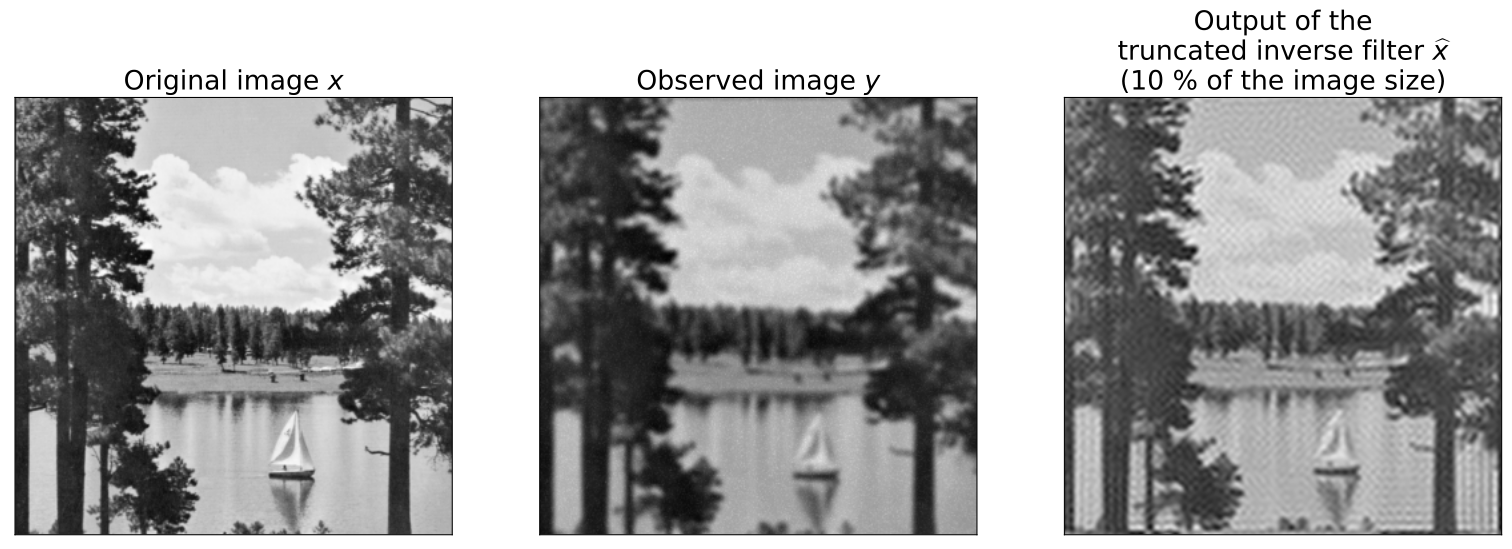
Figure 5:Result of the truncated inverse filter with very small noise.
Wiener Filter
Wiener filter, denoted by (with Fourier transform ), applies to the observation such that:
This filter is established in the statistical framework: the image and the noise are considered to be random variables. They are also assumed to be statistically independent. As a result, the observation and the estimate are also random variables.
The calculations are done in the Fourier domain for simplicity (since convolutions become multiplications). The goal of Wiener filter is to find the image closest to , in the sense of the mean squared error . Thereby :
where is an image filled with 1. So:
where denotes the conjugate of the variables. Since the expectation is linear and only and are random variables, we can decompose the previous expression into four terms:
Since and are independent, then the covariances and are zeros. Moreover, and are the power spectral densities denoted as and (the power spectral density is the expectation of the square of the modulus of the Fourier transform). So the mean squared error simplifies into:
We look for the filter that minimizes the MSE, or equivalently, that cancels the derivative of MSE:
Here we are, we get the expression of the Wiener filter ! 🥳 Finally, the deconvolved image is the inverse Fourier transform of :
We can consider that the power spectral densities and are constant (for , it is necessary to assume white noise). Thus, the expression of the Wiener filter can be written
and the term is replaced by a constant , which becomes the parameter of the method, to be set by the user.
Two remarks:
where vanishes (typically in high frequencies), the problem of noise increase is no longer observed as with the inverse filter, since the inverse filter tends towards 0,
moreover, if the noise in the image is zero, then and Wiener filter comes back to the inverse filter:
The result of Wiener filter is presented Figure 6: it is clearly much better than the inverse filter, even its truncated version!
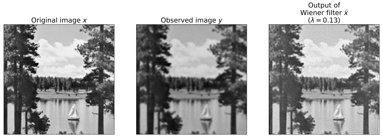
Figure 6:Result of Wiener filter ( is set so that the estimation is the best in terms of MSE).