Filtering aliasing

Aliasing (french: crénelage) is a phenomenon that occurs when the image is poorly sampled. It can be avoided by applying an anti-aliasing filter (french: filtre anti-repliement) before sampling.

Load and display the image roof.jpg. Then, downsample it (without an anti-aliasing filter) by a factor of three by taking one pixel out of three in the two spatial dimensions, which can be done with the instruction
```
f[::3,::3]
```
How does the phenomenon of aliasing appear visually?
Now, apply a Gaussian filter (skimage.filters.gaussian) to the original image before downsampling. Adjust the filter parameter to minimize aliasing. Is the aliasing still visible?
Lastly, replace the Gaussian filter with an ideal low-pass filter, which completely eliminates frequencies above the cutoff frequency without modifying the frequencies below. The process is:
1. Compute the DFT of the image,
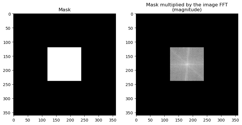
2. Define the ideal filter as a zero image with a square of 1 in the Fourier domain,
3. Multiply the DFT of the image with the filter (this is equivalent to a convolution in the spatial domain),
4. Compute the inverse DFT of the result (and keep only the real part).
The code below generates a binary square mask of the same size as the image X:
```
Mask = np.zeros(X.shape)
Mask[a:b,c:d] = 1
```
Choose correctly the coordinates a, b, c and d to conserve the low frequencies, which are located at the center in the DFT (after applying numpy.fft.fftshift).
The ideal filter may be defined in the same way as in the exercise : use the function numpy.zeros and the indexing f[m1:m2,n1:n2] = x. Choose the cutoff frequency appropriately to reduce aliasing without altering the image. Is the aliasing still visible?

**📌 Commentaires pour les intervenants

Attention, comme il est question de crénelage (aliasing), il ne faut pas afficher les images dans le notebook avec imshow, car les images seront forcément affichées avec un zoom qu’on ne peut pas contrôler, et donc qui risque d’ajouter de l’aliasing... À la place, utiliser l’afficheur Linux de base après avoir enregistré les images, en veillant à avoir un zoom à 100 %. On peut d’ailleurs faire en sorte que cet afficheur soit toujours visible en cliquant sur la barre de titre de la fenêtre avec le bouton droit, puis en sélectionnant « Toujours au premier plan ». Tout ceci sera à faire en point oral aux étudiants.
Un autre point oral à faire : expliquer comment fonctionne le masque à appliquer sur la TFD de l’image. Je pense qu’un petit schéma de ce masque, en expliquant les coordonnées du carré de 1 peut être intéressant.
Pour éviter les problèmes de conversion lors de l’enregistrement des images, utiliser : skimage.img_as_ubyte et .astype(np.uint8).

import numpy as np
import skimage.io as io
import skimage.filters as flt
import matplotlib.pyplot as plt
from skimage import img_as_ubyte

Objectives¶

Define and apply a filter for a real application.
Discover aliasing in images.

Downsampling and filtering¶

Three images are generated:

the original one, rescaled by a factor $S$ ,
the original one, filtered by a Gaussian filter, then rescaled by a factor $S$ ,
the original one, filtered by an ideal low-pass filter (defined in the Fourier domain), then rescaled by a factor $S$ .

Note that when using the inverse Fourier transform, you may have to get the real part of the result, if it is complex.

# Original image
x = io.imread("roof.jpg")

# Scaling without low-pass filtering
y = x[::3,::3]
io.imsave("roof-none.png",y)

# Scaling with Gaussian filtering
x_filtered = flt.gaussian(x, 1.4)
y = x_filtered[::3,::3]
io.imsave("roof-gaussian.png",img_as_ubyte(y))

# Scaling with ideal low-pass filtering, in the Fourier domain

# Image FFT
X = np.fft.fft2(x)
X = np.fft.fftshift(X)

The mask is of the same size that the Fourier transform X of the original image. The low frequencies must be 1 and the high frequency 0, as in the image below (the pixels 1 are in the center to manage the use of fftshift):

# Zero image
M, N = X.shape
Mask = np.zeros((M,N))

# Cutoff frequency (between 0 and 1)
f = .33

# Region where the filter equals 1
a = int(M/2*(1-f))
b = int(M/2*(1+f))
c = int(N/2*(1-f))
d = int(N/2*(1+f))
Mask[a:b,c:d] = 1

X_filtered = X*Mask
X_masked = X_filtered.copy() # for display

# Inverse FFT
X_filtered = np.fft.ifftshift(X_filtered)
x_filtered = np.fft.ifft2(X_filtered)
x_filtered = np.real(x_filtered)
y = x_filtered[::3,::3]

io.imsave("roof-ideal.png",y.astype(np.uint8))

# Display the mask

fig, axs = plt.subplots(1, 2, figsize=(10,5))
axs[0].imshow(Mask, cmap="gray")
axs[0].set_title("Mask")
axs[1].imshow(np.log(np.abs(X_masked)+1e-1), cmap="gray")
axs[1].set_title("Mask multiplied by the image FFT\n(magnitude)")
plt.show()

Note that the cutoff frequency equals $1/S$ to avod aliasing.

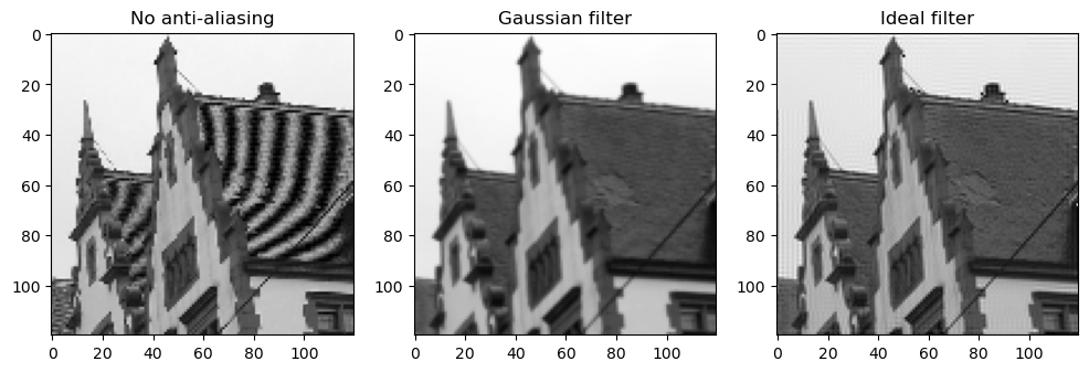
You should obtain the following results. The aliasing is clearly visible on the first image, where no filter has been applied: a weird effect is visible on the tiles. The Gaussian filter strongly attenuates the effect, and the ideal filter is better.

images = ["roof-none", "roof-gaussian", "roof-ideal"]
titles = ["No anti-aliasing", "Gaussian filter", "Ideal filter"]
fig, axs = plt.subplots(1, 3, figsize=(12,5))
for i in range(len(images)):
    x = io.imread(f"{images[i]}.png")
    axs[i].imshow(x, cmap="gray")
    axs[i].set_title(titles[i])
plt.show()