Filtering aliasing

Aliasing (french: crénelage) is a phenomenon that occurs when the image is poorly sampled. It can be avoided by applying an anti-aliasing filter (french: filtre anti-repliement) before sampling.

Warning

Do not display the images in the notebook in this exercise! Jupyter Lab and Matplotlib can create aliasing on display. Instead, save the images with skimage.io.imsave and look at them with an external viewer, by taking care of using a 100% zoom.

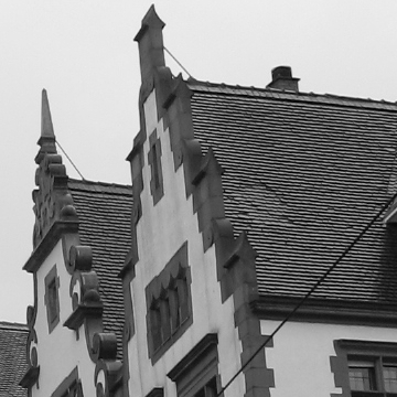
• Load and display the image roof.jpg. Then, downsample it (without an anti-aliasing filter) by a factor of three by taking one pixel out of three in the two spatial dimensions, which can be done with the instruction

  f[::3,::3]
  

  How does the phenomenon of aliasing appear visually?

• Now, apply a Gaussian filter (skimage.filters.gaussian) to the original image before downsampling. Adjust the filter parameter to minimize aliasing. Is the aliasing still visible?

• Lastly, replace the Gaussian filter with an ideal low-pass filter, which completely eliminates frequencies above the cutoff frequency without modifying the frequencies below. The process is:

  1. Compute the DFT of the image,

  2. Define the ideal filter as a zero image with a square of 1 in the Fourier domain,

  3. Multiply the DFT of the image with the filter (this is equivalent to a convolution in the spatial domain),

  4. Compute the inverse DFT of the result (and keep only the real part).

  The code below generates a binary square mask of the same size as the image X:

  Mask = np.zeros(X.shape)
  Mask[a:b,c:d] = 1
  

  Choose correctly the coordinates a, b, c and d to conserve the low frequencies, which are located at the center in the DFT (after applying numpy.fft.fftshift).

  The ideal filter may be defined in the same way as in the exercise Create a simple image: use the function numpy.zeros and the indexing f[m1:m2,n1:n2]=x. Choose the cutoff frequency appropriately to reduce aliasing without altering the image. Is the aliasing still visible?

Correction

Objectives

• Define and apply a filter for a real application

• Discover aliasing in images

Warning

Because Jupyter Lab and Matplotlib show images with a rescaling, the function imshow can introduce aliasing, even if there is no aliasing in the actual image. Therefore, do not use imshow in this exercice, but save the image (with skimage.io.imsave) and display it by using an external viewer.

Downsampling and filtering

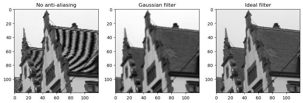
Three images are generated:

• the original one, rescaled by a factor \(S\),

• the original one, filtered by a Gaussian filter, then rescaled by a factor \(S\),

• the original one, filtered by an ideal low-pass filter (defined in the Fourier domain), then rescaled by a factor \(S\).

Note that when using the inverse Fourier transform, you may have to get the real part of the result, if it is complex.

The mask is of the same size that the Fourier transform X of the original image. The low frequencies must be 1 and the high frequency 0, as in the image below (the pixels 1 are in the center to manage the use of fftshift):

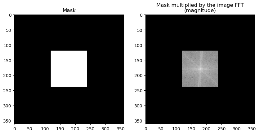
Note that the cutoff frequency equals \(1/S\) to avod aliasing.

You should obtain the following results. The aliasing is clearly visible on the first image, where no filter has been applied: a weird effect is visible on the tiles. The Gaussian filter strongly attenuates the effect, and the ideal filter is better.