Convolution#
The image smiley.png will be convolved with several PSF.
Before applying the convolutions, you need to convert the image into float (skimage.img_as_float).
Note
It can be very useful for analyzing the results to display the colorbar alongside each image.
You can follow the code below
(img is the image to show):
import matplotlib.pyplot as plt

plt.figure()
ax = plt.imshow(img, "gray")
plt.colorbar(ax)
plt.show()
What does the acronym PSF stand for?
Compute the convolution between the image and a Gaussian kernel (
skimage.filters.gaussian).Compute the convolution between the image and the kernel defined by
\[ h = \begin{pmatrix} 1 & -1 \end{pmatrix}, \]by using
scipy.ndimage.convolveand initializing \(h\) withnumpy.array. Note that \(h\) being an image, it should be defined as a 2D matrix!Compute the convolution between the image and a kernel defined by an array of 30 elements equal to 1/30 (
numpy.ones).
Correction#
Objectives#
know how to use the function
scipy.ndimage.convolveto apply the convolution productbe able to identify the kernel applied on a convolved image
The point spread functions#
Before convolving the image by the different filters, it is interesting to display the filters themselves.
In case there is no explicit matrix to represent a filter, as with the Gaussian filter skimage.filters.gaussian,
we can simply convolve the filter by an image containing only one non-zero pixel.
Indeed, this image is equivalent to a Dirac pulse \(\delta\) which is the neutral element of the convolution product.
The two last kernels are defined with (note the double brackets, so as to get a 2D array):
h = np.array([[1, -1]])
and
N = 30
h = np.ones((1,N)) / N
The convolutions#
The results of the convolutions are shown below, for both the “Dirac pulse” (first row) and the smiley (second row).
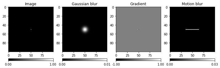
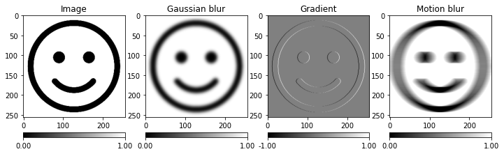
The function skimage.filters.gaussian defines a Gaussian kernel (this is the second image above).
The result of the function is the convolution product of this Gaussian kernel with the image given as a parameter of the function.
The “gradient” image (third image) brings out the vertical contours of the image. We will reuse this filter in Edge detection.