L’année dernière, les étudiants n’ont abordé que le débruitage.
Le déconvolution ne sera donc abordée que par les étudiants les plus rapides.
Ce n’est pas grave, d’autant plus que l’exercice sur la déconvolution est similaire à celui sur le débruitage.
il me semble important que les étudiants sachent simuler une observation, c’est-à-dire générer le modèle direct.
En effet, c’est une manière classique de produire des données et la solution recherchée.
C’est pour cela que les premières questions, loin d’être anodines, leur demande de générer une image bruitée ou floutée.
La correction que je propose ci-dessous est très complète : je n’attends pas autant des étudiants.
Il faut continuer à pousser les étudiants à développer leur esprit critique.
Cela commence par faire une bonne observation des résultats obtenus, à faire une interprétation correcte,
à proposer des solutions pour améliorer la méthode où pour aller plus loin dans la compréhension du problème,
et enfin à proposer de nouvelles expériences pour vérifier les hypothèses émises.
This exercise is intended to evaluate the performances of the denoising method of your choice.
Therefore it is essential to have an image corrupted by noise and the same image without noise
to be able to compare the denoising method with the actual image.
In the case of an AWGN,
the power of the noise is a good estimation of the variance of the Gaussian.
Express the Gaussian variance σ2 in terms of SNR.
Add noise to the image of your choice by using skimage.util.random_noise
(with parameter clip=False to get a real Gaussian noise).
Check that the noise level corresponds to the expected SNR.
For example, noise should be barely visible above 30 dB.
On the contrary, the image should be difficult to discern below 0 dB.
Now that you dispose of a noisy image and its noiseless version,
you can implement the denoising method.
Denoise the image with the chosen method:
If you choose a mean filter, use scipy.ndimage.convolve to filter by a square PSF
h = np.ones((w,w)) / (w*w) of size w.
If you choose TV regularization, use skimage.restoration.denoise_tv_chambolle.
Observe visually the effect of the parameter (size of the mean filter or regularization parameter) on the result, especially for extreme values.
Use skimage.metrics.mean_squared_error
to calculate the mean squared error (MSE, in French EQM for erreur quadratique moyenne)
of the denoised image to have a quantitative measure of the denoising quality.
Represent the evolution of the MSE according to the parameter, and comment on the result:
what is the optimal value of this parameter?
Can you adjust the parameter by knowing the SNR of the image?
Compare your method with the one implemented by another student.
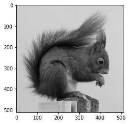
x = imread("squirrel.png")
x = x.astype(float)
M, N = x.shape
imshow(x, cmap="gray")
show()
The signal-to-noise ratio (SNR) is defined as the power of the image x divided by the power of the noise b.
Besides, it is generally given with a logarithmic scale.
Note that ∑m,nx(m,n)2 corresponds to the Frobenius norm of x and can be calculated with numpy.linalg.norm.
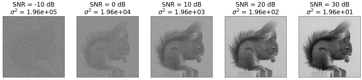
The figures below represent the image at different noise levels.
Warning: do not forget clip=False when using skimage.util.random_noise, in order to add a true Gaussian noise!
rsbs = [-10, 0, 10, 20, 30]

figure(figsize=(25,10))
i = 0

for rsb in rsbs:
    var = variance(rsb, x)
    y = random_noise(x, mode='gaussian', clip=False, var=var)
    # print(x.min(), x.max())
    # print(y.min(), y.max())
    i = i + 1
    subplot(1,5,i)
    imshow(y, cmap="gray")
    xticks([])
    yticks([])
    title(f"SNR = {rsb:.0f} dB\n$\sigma^2$ = {var:.2e}", fontsize=24)
Note that the larger the SNR, the less visible the noise.
This makes sense since, in the definition of SNR, the noise power is in the denominator.
In addition, the noise becomes almost invisible beyond 30 dB, while it is very high and the image is hardly visible below 0 dB.
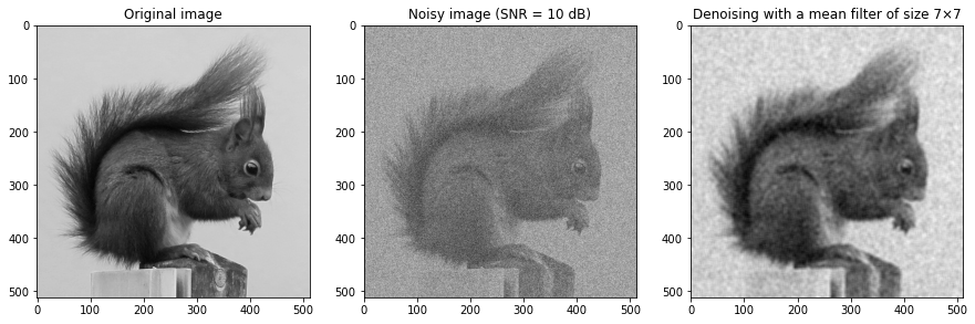
I choose the image whose SNR equals 10 dB, and I apply a mean filter.
snr = 10
var = variance(snr, x)
y = random_noise(x, mode='gaussian', clip=False, var=var)
# Exemple d'un filtre moyenneur pour une taille particulière
w = 7
h = ones((w,w)) / (w*w)
xest_mean = convolve(y, h)

# Affichage
figure(figsize=(15,5))
subplot(1,3,1)
imshow(x, cmap="gray")
title("Original image")
subplot(1,3,2)
imshow(y, cmap="gray")
title(f"Noisy image (SNR = {snr} dB)")
subplot(1,3,3)
imshow(xest_mean, cmap="gray")
title(f"Denoising with a mean filter of size {w}×{w}");
We observe that the mean filter reduces the noise, which is expected (have you tried a filter of size 1×1? What’s going on?).
On the other hand, the image is more blurry: the contours are less sharp.
This second observation is explained by the fact that the mean filter is a convolution by a kernel which is not a single pulse:
so the intensities of the pixels spreads over their neighbourhood.
The mean squared error is an objective measure of the quality of the restoration.
It is calculated between the denoised image x^ and the original one x.
Therefore, the mean filter helps to decrease the MSE by reducing the noise.
But at the same time it increases the MSE by introducing blur in the image.
As a consequence, the MSE evolves with the size w×w of the filter.
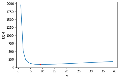
To verify this hypothesis, we plot the values of the MSE with respect to w:
# Évolution de l'EQM en fonction de la taille du filtre
ws = arange(1,40)
mses = zeros(ws.shape)
for i, w in enumerate(ws):
    h = ones((w,w)) / (w*w)
    xest = convolve(y, h)
    mses[i] = mean_squared_error(x, xest)
i = argmin(mses)
mse = mses[i]
w = ws[i]

plot(ws, mses)
plot(w, mse, 'r.')
xlabel('w')
ylabel('EQM')
show()
As expected, the MSE change with respect of the filter size.
A compromise must be made between the noise reduction and the blurring.
We observe that the curve has a minimum, it corresponds to the best choice for w (in terms of MSE).
print(f"The best restoration is obtained for w = {w:.0f} and get an MSE = {mse:.2e}")
The best restoration is obtained for w = 9 and get an MSE = 8.21e+01
Unfortunately, there is no easy way to know a priori the best size of the mean filter just knowing the SNR.
The value obtained here depends on the image (try with another image!).
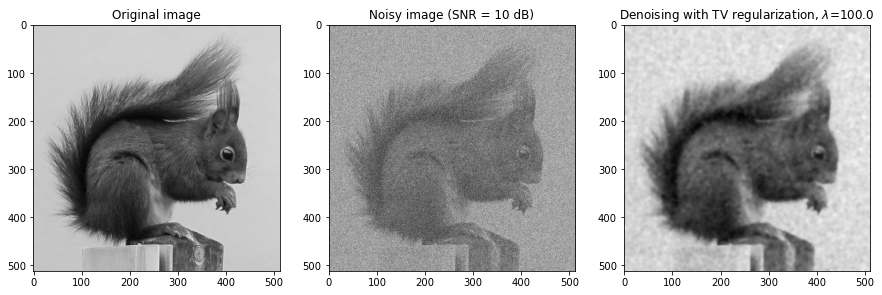
As with the mean filter, we observe that the image is partially denoised (therefore the MSE will be better),
but, again, the contours are less sharp, resulting in a degradation of the MSE.
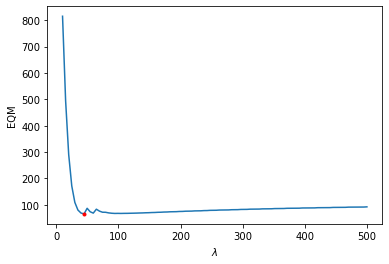
As previously, it should exist an optimal value of the regularization parameter λ.
Let’s see if this denoising technique can surpass the mean filter...
# Évolution de l'EQM en fonction de la taille du filtre
lbds = linspace(10, 500, 100)
mses = zeros(lbds.shape)
for i, lbd in enumerate(lbds):
    xest = denoise_tv_chambolle(y, weight=lbd)
    mses[i] = mean_squared_error(x, xest)
i = argmin(mses)
mse = mses[i]
lbd = lbds[i]

plot(lbds, mses)
plot(lbd, mse, 'r.')
xlabel('$\lambda$')
ylabel('EQM')
show()

print(f"The best restoration is obtained for lambda = {lbd:.0f} and get an MSE = {mse:.2e}")
The best restoration is obtained for lambda = 45 and get an MSE = 6.51e+01
The curve has the same behavior as in the case of the mean filter:
there is an optimal value of the regularization parameter for which the MSE is the best.
Moreover, we notice that the best MSE is lower than the best MSE obtained with the mean filter.
So we want to conclude that TV regularization is more efficient than the mean filter!
But beware: this conclusion is partial, because it was only obtained on one image with one SNR.
Comparison of the two denoising methods for different SNRs
It is possible to analyze the evolution of the MSE with respect to the noise level by calculating, for several values of SNR,
the best parameters for the two methods.
rsbs = arange(-5, 20, 2)

# Filtre moyenneur
ws = arange(1,40)
mean_eqm = zeros(rsbs.shape)
mean_w = zeros(rsbs.shape)

# Régularisation TV
lbds = linspace(0, 200, 20)
tv_eqm = zeros(rsbs.shape)
tv_lbd = zeros(rsbs.shape)

for i, rsb in enumerate(rsbs):

    # Génération de l'image bruitée
    var = variance(rsb, x)
    y = random_noise(x, mode='gaussian', clip=False, var=var)

    # Filtre moyenneur
    besteqm = inf
    for w in ws:
        h = ones((w,w)) / (w*w)
        xest = convolve(y, h)
        eqm = mean_squared_error(x, xest)
        if eqm < besteqm:
            besteqm = eqm
            bestw = w
    mean_eqm[i] = besteqm
    mean_w[i] = bestw

    # Débruitage TV
    besteqm = inf
    for lbd in lbds:
        xest = denoise_tv_chambolle(y, weight=lbd)
        eqm = mean_squared_error(x, xest)
        if eqm < besteqm:
            besteqm = eqm
            bestlbd = lbd
    tv_eqm[i] = besteqm
    tv_lbd[i] = bestlbd
/home/vincent/anaconda3/lib/python3.9/site-packages/skimage/restoration/_denoise.py:431: RuntimeWarning: divide by zero encountered in scalar divide
  norm *= tau / weight
/home/vincent/anaconda3/lib/python3.9/site-packages/skimage/restoration/_denoise.py:431: RuntimeWarning: invalid value encountered in multiply
  norm *= tau / weight
Then we can represent the evolution of the MSE for the two methods:
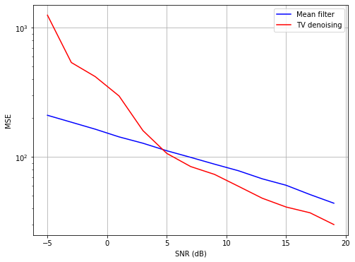
We observe that the MSE decreases with the SNR.
The interpretation is easy:
the more the noise decreases, the more the image resembles the original image, and therefore denoising is less difficult.
In addition, we observe that:
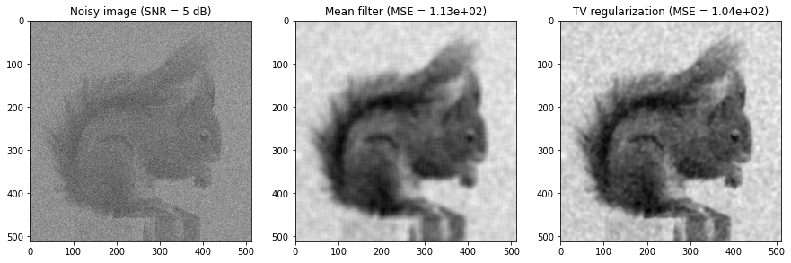
for SNRs lower than (approximately) 5 dB, the mean filter is better than TV regularization.
This seems surprising since the TV regularization is supposed to be better.
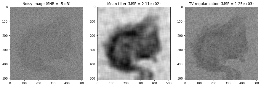
However, an SNR lower than 5 dB is extremely low.
In fact, neither of the two methods gives a really satisfactory result (see below).
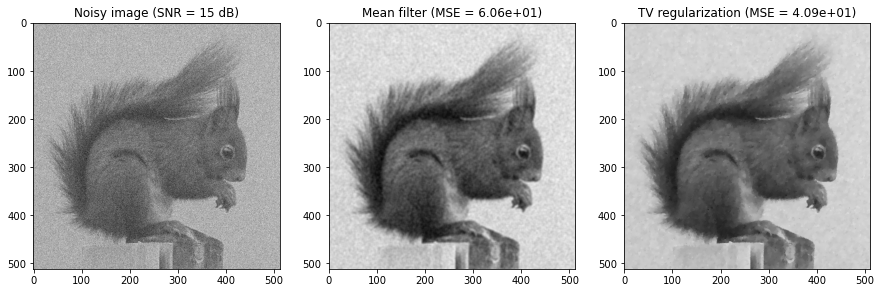
for images with SNR greater than 5 dB, TV regularization is better.
idx = [0, 5, 10]

for i in idx:

    rsb = rsbs[i]

    # Génération de l'image bruitée
    var = variance(rsb, x)
    y = random_noise(x, mode='gaussian', clip=False, var=var)

    # Filtre moyenneur
    w = int(mean_w[i])
    h = ones((w,w)) / (w*w)
    xest_mean = convolve(y, h)
    eqm_mean = mean_squared_error(x, xest_mean)

    # Débruitage TV
    lbd = tv_lbd[i]
    xest_tv = denoise_tv_chambolle(y, weight=lbd)
    eqm_tv = mean_squared_error(x, xest_tv)

    # Affichage
    figure(figsize=(15,15))
    subplot(1,3,1)
    imshow(y, cmap="gray")
    title(f"Noisy image (SNR = {rsb} dB)")
    subplot(1,3,2)
    imshow(xest_mean, cmap="gray")
    title(f"Mean filter (MSE = {eqm_mean:.2e})")
    subplot(1,3,3)
    imshow(xest_tv, cmap="gray")
    title(f"TV regularization (MSE = {eqm_tv:.2e})")
OK, we have the same conclusions as before.
The comparison between the two methods was only carried out on a single image and a single criterion (the MSE).
This is undoubtedly a good criterion for comparing two methods, but other criterions exist,
such as for example the complexity of the method, the computation time, etc.